- Anyons Motivation
- Braid Group
- The Braid Group & Yang Baxter Equation
- Hecke Algebra
- Appendix A: Quotient & Kernel of Groups
- Appendix B: Local Representation of Hn(q)
- Appendix C: Cayley-Hamilton Theorem
- Sources
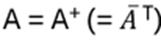
Anyons Motivation [1]
In the following series the connection of topology and Anyons will be shown. The quantum computing ‚relevant‘ part are the Anyons, but they will come last. Since some (actually a lot) topology lies ahead, I start with the Anyons, which will be explained in more detail later, but having a first glimpse in mind is maybe helpful when introducing the Braid Group, the YBE and Quantum Groups, etc. So, let’s start with a not thoroughly introduction of Anyons:
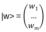
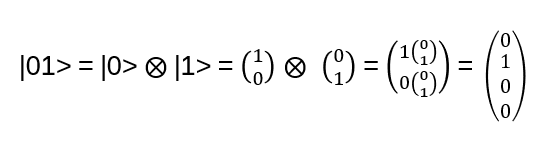
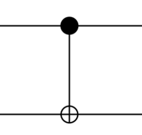
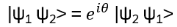
Exchanging two undistinguishable particles gives
|ψ1 ψ2> = ± |ψ2 ψ1>, depending if the particles are Bosons or Fermions.
Thinking in terms of paths, 2 particles changing from ‘configuration’ 1 to 2 in strictly two dimensions looks like:
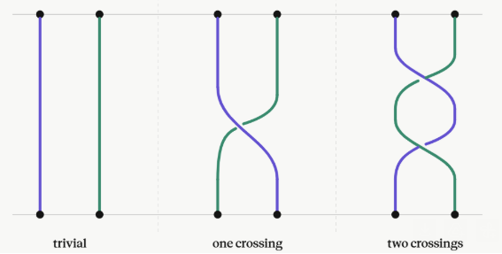
In two dimensions, no exchange path can be contracted to the trivial path on the left without additional crossings.
Interpreted as the 2+1-dimensional spacetime: in 3 spatial dimensions, the loop of particle B encircling particle A can be continuously deformed to a point. In 2 dimensions, this is not possible and a particle B winding around A once is topologically different to winding around twice!
For such particles it holds:
with arbitrary

in R (being 0 for Bosons, π for Fermions), hence the name ‘Any’-ons.
The movement on Anyons in 2+1 dimensions is given by the Braid Group (details will follow), with generators obeying
bibj = bjbi for | i – j | > 1
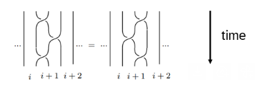
bibi+1bi = bi+1bibi+1 for 1 ≤ i ≤ n-1
or represented by strands, where the b’s causing the exchange, e.g.
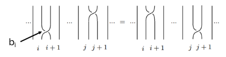
or
Those particles are called quasi particles:
- They are not point particles, but vortex-like disturbances spread across many electrons, i.e. anyons arise as collective excitations of multiple particles
- They are strictly 2 dimensional: the electrons live in a thin layer
- Without going into details, the following is just cited here as a remark, that the above is not just theory: using Quantum Hall regimes, braiding one quasi particle around another leads to the Aharonov–Bohm phase, which is the anionic phase mentioned above, e.g. [2]!
The very high-level summary of what I will look into in the course of this blog series:
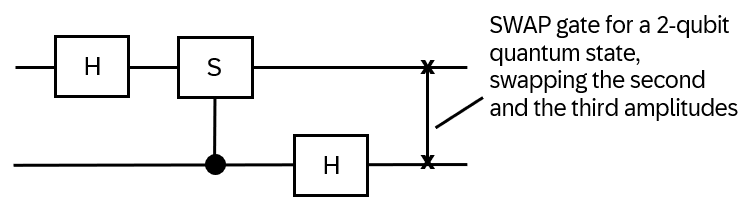
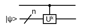
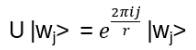
The defining equation for the Braid group on strands satisfies the Yang-Baxter Equation. Use R-matrices (solutions to the YBE, swapping strands and resulting in braids ) to represent anyon interactions and braids will turn out to be quantum gates on anyon pairs!
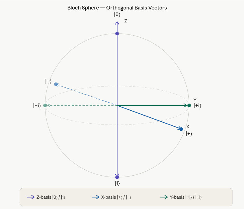
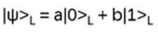
Exchanging (non-abelian) anyons in 2-dimensional systems gives the corresponding wave function a phase (represented by a unitary operator, [3], e.g. Fibonacci anyons or Majorana zero modes). Braiding those anyons applies the unitary matrices to a degenerate groundstate subspace and that subspace encodes a qubit!
The topological protection comes from the fact that only the braid (which strand went over which) matters, not microscopic perturbations. A local error can’t change the topology of a worldline, without braiding an anyon around another, which would be a macroscopic, detectable event!
Braid Group [4]
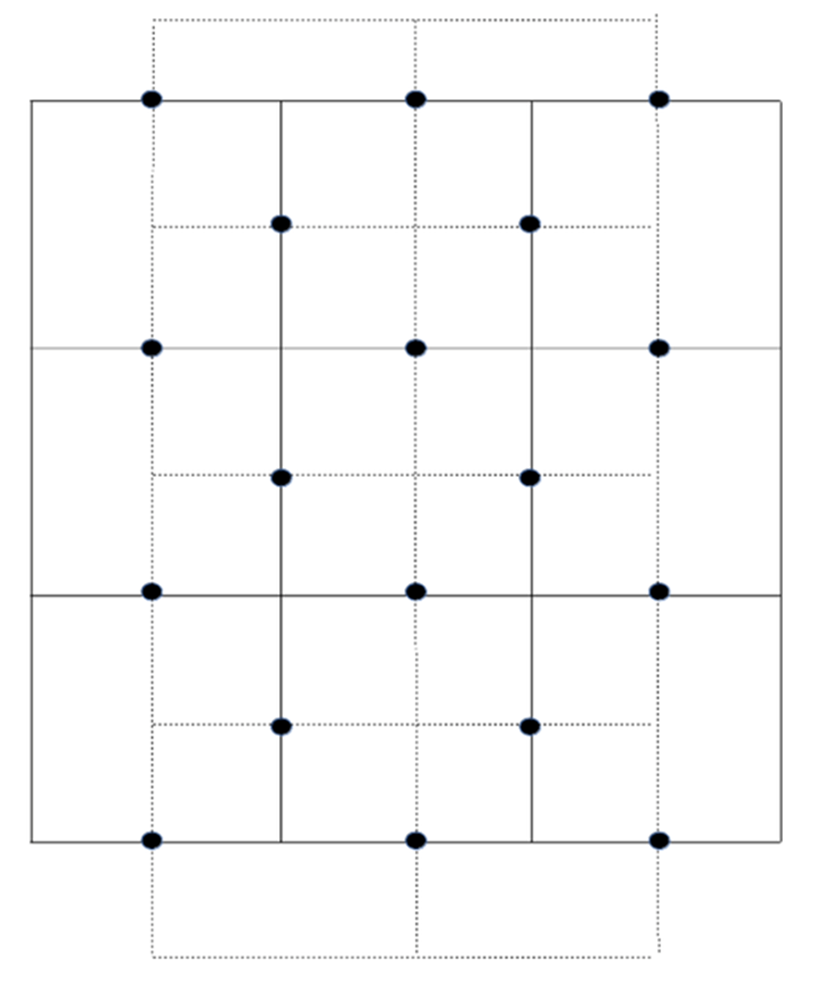
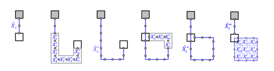
A braid on n strands (or strings) is an object of 2n points connected by n strings such that
i. The strings begin and end all at the 2n points above and below, e.g.
ii. No string intersects any horizontal line more than once
iii. The strings do not intersect, e.g. here are two projections from three dimensions:
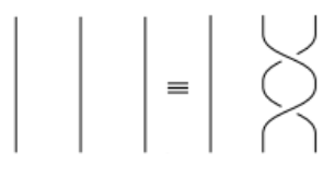
Two strings are equivalent if the strings can be continuously deformed without crossing into each other, e.g.
Bn := all braids up to equivalence on n strings. Define an add operation:
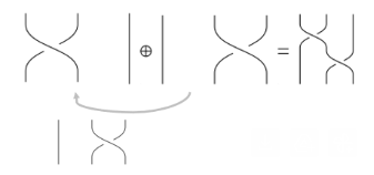
(Bn ,+) forms a group
Examples:
- B1 = trivial group
- B2 = with strings there is only one possible crossing, hence the questions are essentially ‘how many crossing’ and ‘which direction’. E.g.
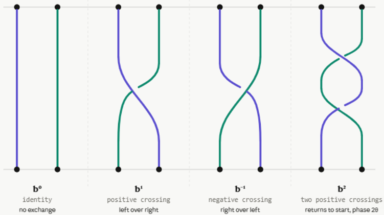
Hence B2 has one generator with the identity b0, b1 anticlockwise crossing, b-1 clockwise crossing, and the inverse b+1b-1 = b0. This is equivalent (isomorph) to (N,+), integers with the + operator, counting the crossings
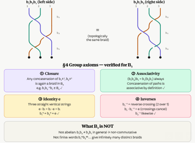
- B3: this group is infinite and non-abelian (non-commutative)! What are the generators of B3?
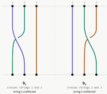
B3 = <b1, b2> and each braid can be associated with a permutation of {1, 2, 3}. Emil Artin proved in 1925 ([5, from 1947]), that b1b2b1 = b2b1b2 as the fundamental relationship between b1 and b2; there are no other relations like b12 and e (identity element) or b22 and e. Hence the summary:
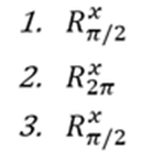
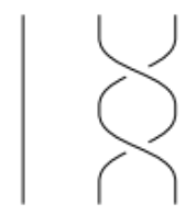
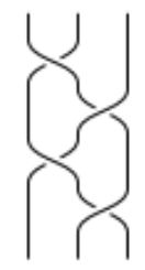
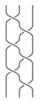
Are there braids which commute with all others? Yes, e.g. (b1b2)3, representing a full twist of a string:
The Braid Group & Yang-Baxter Equation [6]
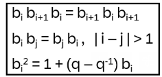
The braid group Bn is generated by b1, …, bn-1 and following relations:
bi bi+1 bi = bi+1 bi bi+1
bi bj = bj bi for | i – j | > 1
Let V be a vector space,

the tensor product on V. Define operators R1, …, Rn-1 so that
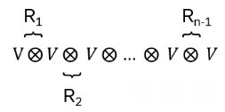
I.e.: Ri acts on
non-trivially only on the i – and i+1 – V-’components’:
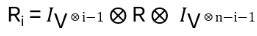
(note the dimensions: i-1+n-i-1=n-2, R acting on two V!)
R defines a ‘local representation’ of Bn on the tensor space
with
if the braid relation is fulfilled:
From the locality of Ri, Rj the other relation follows: RiRj = RjRi if |i–j| > 1
( Recall: End = endomorphism, i.e. all linear maps on itself. Example:
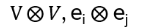
building the basis having 4 dimensions: {e1 e1 , e1
e2 , e2
e1 , e2
e2}. Now,
are n2xn2 matrices:

i.e. 24 basis matrices )
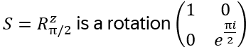
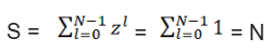
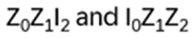
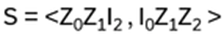
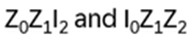
S be in
then define Sij as an operator on

with
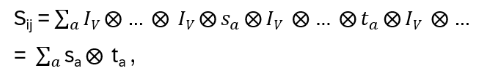
sa at the ith, ta at the jth position with sa, ta in End(V). Use this notation for the permutation operator P on
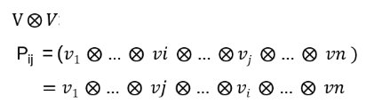
Recall the transposition operator πij(k): k = j if k equals i and k = i if k equals j and else k. Then it holds:
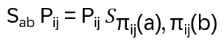
Examples: a) S13P12 = P12S23 , b) P23S12P23 = S13
Define
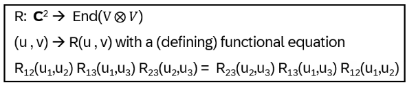
with the operators acting on
This is the Yang-Baxter equation! It is a consistency characteristic of a system if it holds
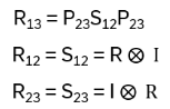
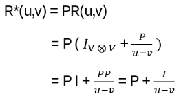
From the ‘algebraic’ version of the YBE above, derive the ‘braided’ one:

P being the permutation operator from above
Define R1*(u,v) := R12*(u,v) and R2*(u,v) := R23*(u,v). Then the YBE reads
R1*(u1,u2) R2*(u1,u3) R1*(u2,u3) = R2*(u2,u3) R1*(u1,u3) R2*(u1,u2)
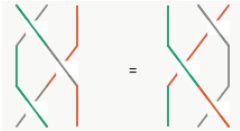
This is the braid relation from the local representation of Bn from before! In the braid view, it says for 3 strands, pulling a strand past a crossing doesn’t change the overall braid
Example: show that
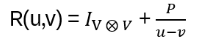
satisfies the algebraic YBE. First note: if this is true, then
is a solution to the braided version of the YBE!
Define a := u-v, b = u, c = v, a = b-c. Why? R is invariant against a shift λ: R(x-y) = R[ (x+ λ) – (y+ λ) ] and hence R(u,v) depends only on the difference u-v. Therefore, Rij actually depends only on two parameters! Choose u3 = 0
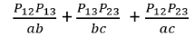
With that: R12(a) = I + P12 / a , R13(b) = I + P13 / b , R23(c) = I + P23 / c
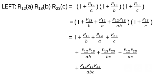
The first lines of the results are identical. Now, use the following identities:
With those: LEFT
multiplied by abc:
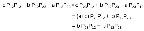
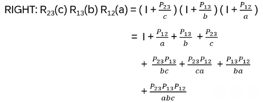
RIGHT analogously …
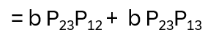
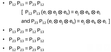
Hence remaining to show: P12P23 =P23P13
P12P23 : (i,j,k)→(i,k,j)→(k,i,j) and P23P13 : (i,j,k)→(k,j,i)→(k,i,j) !
For the ‘abc’ term: P12P13P23 = (i,j,k)→(i,k,j)→(j,k,i)→(k,j,i) and P23P13P12 = (i,j,k)→(j,i,k)→(k,i,j)→(k,j,i)
QED
Hecke Algebra
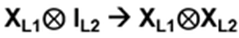
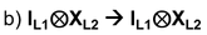
With the braid group an arbitrary number of crossings between strings is possible. Is it possible to add a relation in order to deal with the crossings? Add the relation
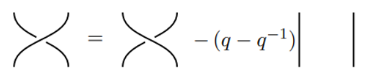
with q in C not zero. This defines the Hecke algebra Hn(q)
The relation above translates to bi-1 = bi – (q – q-1) for all generators bi of the Braid group. Hence the defining relations for Hn(q)
Hn(q) is a quotient of the group algebra of the Braid group Bn with the characteristic equation (bi – q)(bi + q-1) = 0 (see Appendix A: Quotient & Kernels of Groups):
To see this:
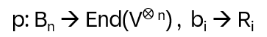
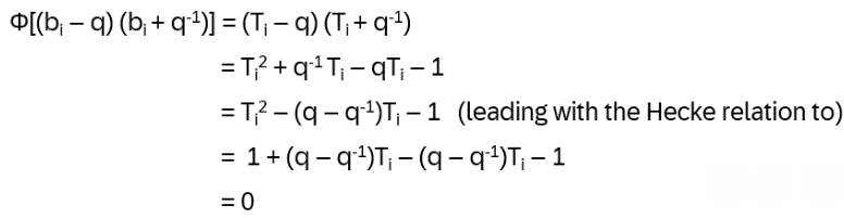
Define Φ: C Bn → Hn(q) , Φ(bi) = Ti with Φ(bibi+1bi) = TiTi+1Ti , Φ(bi+1bibi+1) = Ti+1TiTi+1 , Φ(bi bj) = Ti Tj = Tj Ti = Φ(bj bi) for | i – j | > 1
Every element of Hn(q) is a linear combination of products T1, …, Tn-1 and hence Φ reaches every element in Bn and all elements fᵢ =(bᵢ – q)(bᵢ + q-1) are nonzero in C[Bₙ]. Now form the two sided ideal Id =C[Bₙ]fᵢ C[Bₙ] with elements of the form Σⱼ xⱼ · fᵢ · yⱼ, for all xⱼ, yⱼ ∈ C[Bₙ]. Does x · u ∈ Id and u · x ∈ Id hold in order to be ideal? Yes, because x·(bᵢ – q)(bᵢ + q-1)·y is always a multiple of fᵢ and hence still in Id! Note: that’s the difference to a mere subspace, only closed under addition and scalar multiplication.
With this ideal the quotient Hₙ(q) = C[Bₙ] / Id forces every fᵢ = 0 in the quotient, meaning: (Tᵢ – q)(Tᵢ + q-1) = 0 in Hₙ(q) (because of the additional characteristic equation, not available in C[Bₙ]):
So, (bi – q) (bi + q-1) is in Ker(Φ) for all i, and hence the entire ideal (generated by fᵢ) Id = <(bi – q) (bi + q-1)> is in Ker(Φ)
What is the inverse Ti-1? Ti2 = (q – q-1)Ti + 1 , hence Ti = (q – q-1) + Ti-1, leading to Ti-1 = Ti – (q – q-1)
Check: TiTi-1 = (Ti2 – (q – q-1) Ti) = Ti (q – q-1) + 1 – (q – q-1) Ti = I. With the first isomorphism theorem (see Appendix A) follows with the homomorphism
Φ: C[Bn] → Hn(q): C[Bn] / Ker(Φ) = Hn(q)
Intuitively: in Bn, the generator bi has infinite order, i.e., one can braid bi without ever coming back to the identity. But with the Hecke relation (Ti – q) (Ti + q-1) = 0 in the quotient, Ti is restricted to two eigenvalues, q (the ‘positive’ crossing) and – q-1 (the ‘negative’ crossing). This maps the infinite dimensional braid space of bi into a finite algebraic object, while preserving the full braiding topology, encoded in the YBE!
Note: Sometimes the characteristic equation of Hn(q) is shown as (bi – q)(bi + 1) = 0. By substitution of bi → bi one can show that both are valid (although different) representations of the Hecke algebra by rescaling. They define isomorphic algebras: (bi – q)(bi + 1) = 0 → (
bi – q) (
bi + 1) = 0 → q(bi –
) (bi +
) = 0 Rescale
→ q gives the result
A further characteristic of the Hecke algebra is its connection to the symmetric group Sn: for q2 = 1 one gets Ti2 = 1 and Hn(1) = C[Sn]. It holds not only for q = 1 but all q not equal to zero, that Hn(q) has dimension n!, the same as C[Sn]. In this sense q is ‘deforming’ the algebra smoothly but not changing the size
Another effect of q2 = 1 is that all the topological information is lost, since from the local Hecke relation there is no difference in the crossing anymore (since bi = bi-1) and hence a braid just becomes the permutations of the n points connected by the strings
The braided YBE is satisfied in Hn(q): define
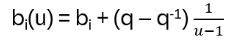
With that the braided YBE follows:
bi(u) bi+1(uv) bi(v) = bi+1(v) bi(uv) bi+1(u)
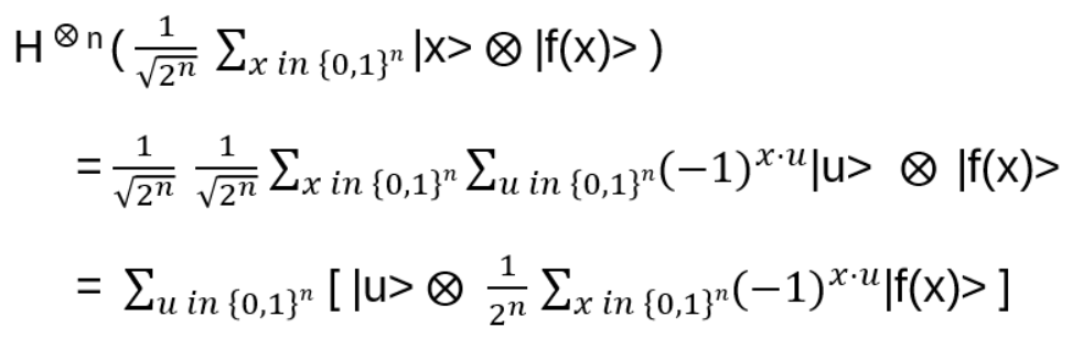
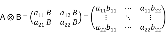
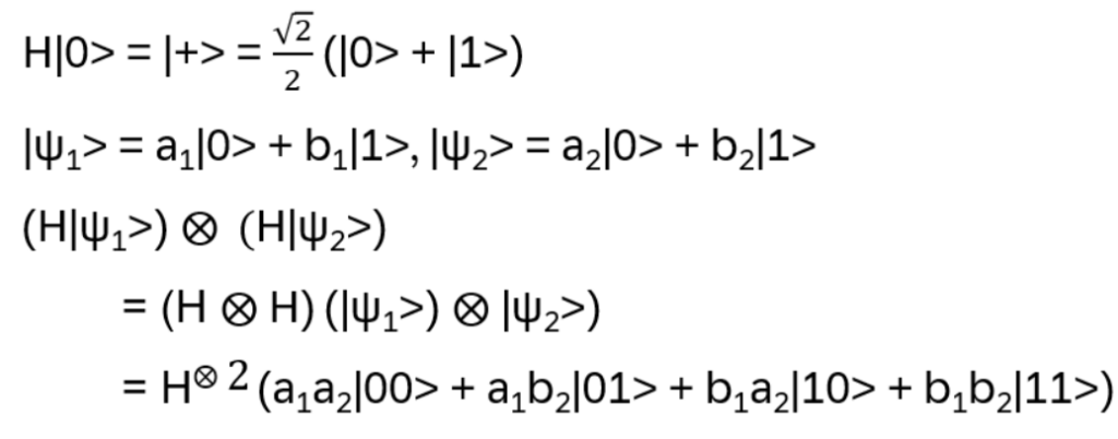
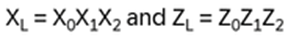
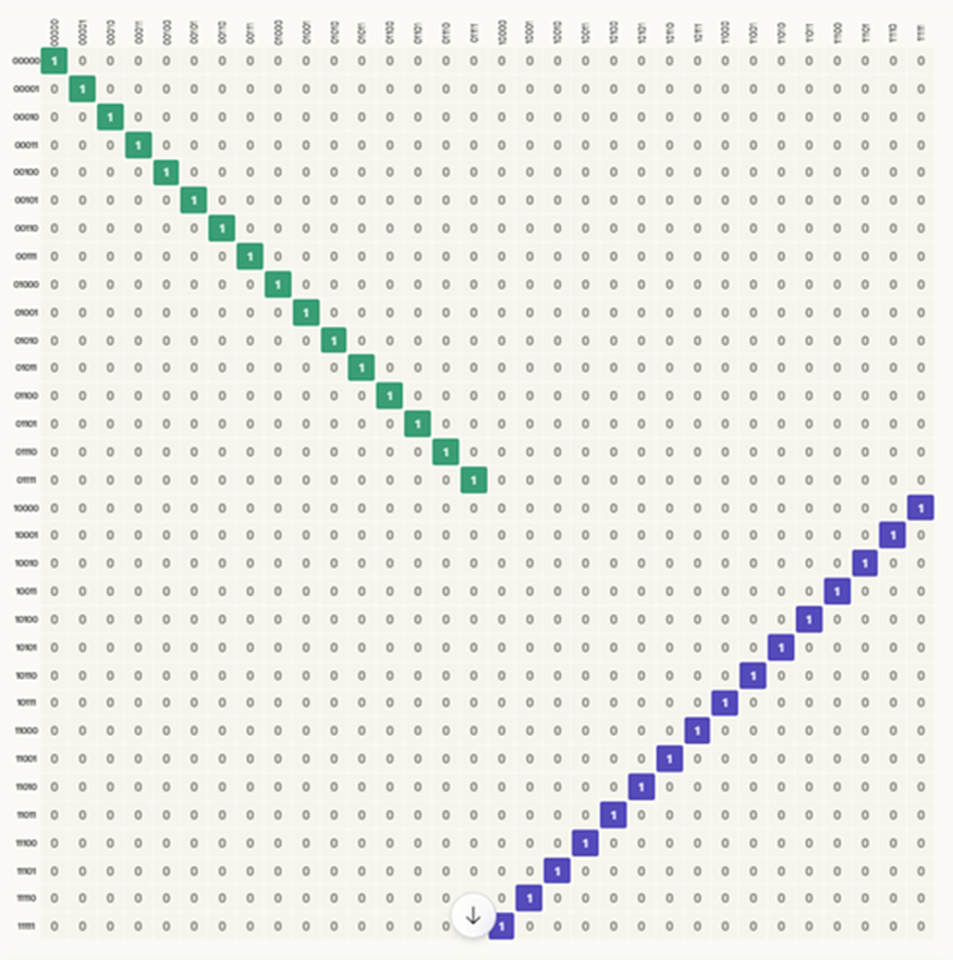
Nice, but since in the end it should be relevant for quantum computing, strings and string crossings may be a bit awkward … where are the orthogonal basis vectors of a Hilbert space? What is needed is a representation of the operator on a tensor product of vector spaces, i.e. a representation of Hn(q) with a specific linear map
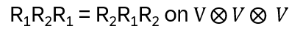
with explicit matrix entries Rijkl, satisfying (R⊗I) (I⊗R) (R⊗I) = (I⊗R) (R⊗I) (I⊗R) for every input vector v₁⊗v₂⊗v₃ ∈ V⊗V⊗V
Notes
- (R⊗I) (I⊗R) (R⊗I) = (I⊗R) (R⊗I) (I⊗R): R lives on V⊗V, but the YBE on V⊗V⊗V (three strings in the braided version), hence I is telling which V-’component’ to keep alone when applying R
- (See later): Quantum groups produce representations of Hn(q) and hence can generate R-matrices, which satisfy the vector space YBE (because the representation homomorphism preserves all relations of an algebra and bi satisfies the braid YBE)
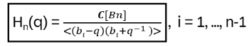
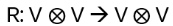
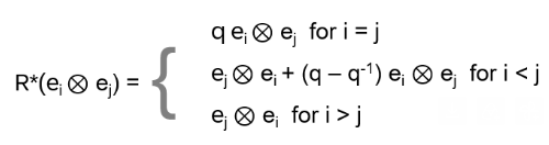
We are looking for a local representation of Hn(q) of the form

I.e. every generator bi is mapped to the same matrix R*, just acting on the (local) components i and i+1. Therefore R* itself is independent of i. It’s translation invariant, the same along the chain
How to find a representation for R*? It turns out: for any V set a basis (e1, …, eN) and define on V⊗V
i, j = 1, …, N. This is a local representation of the braid group: Ri* Ri+1* Ri* = Ri+1* Ri Ri+1* (see Appendix B).
Note: In german there is a saying for something totally unexpected – ‚it is falling from the sky‘ … , but actually R* is not. The R*-matrix defined as above comes from the quantum group Uq(gln), which is a q-deformation of the universal enveloping algebra U(gln), where gln is the Lie algebra of the general linear group GLn (the group of invertible nxn matrices) and it can be derived using the quantum double construction … , [7]. No idea what any of this means? I hope the next blog ‚Topological Quantum Computing II‘ will clarify it!
Now back: this representation factors through the Hecke algebra, since the Hecke relation
is satisfied. In other words: R* lives purely on the reduced quotient of the Braid group (by mapping the extra relation (bi – q)(bi + q-1) of Bn to zero), which is exactly the Hecke algebra.
So, we have a solution of the braided YBE on any vector space!
Appendix A: Quotient & Kernels of Groups
First introduce cosets [8]
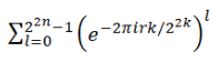
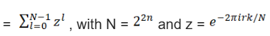
Start with an example: (U13, · ) = {1, 2, 3, …, 12}, H be the subgroup {1, 3, 9}. Choose 6 from U13. Then the coset 6H is obtained by multiplying each element of H by 6:
6H = {6 · 1, 6 · 3, 6 · 9} mod 13 = {6, 5, 2}. Calculate all cosets 1H, 2H, … and take into account that e.g. 4H = {4, 12, 10} = 10H = 12H, the one ends up with 4 distinct cosets:
- 1H = 3H = 9H = {1, 3, 9}
- 2H = 5H = 6H = {2, 5, 6}
- 4H = 10H = 12H = {4, 10, 12}
- 7H = 8H = 11H = {7, 8, 11}
Notes: Only 1H is itself a (sub-) group, because of the identity element. For the coset aH, a is always an element of the coset. All cosets have the same size.
The distinct cosets form a partition of U13!
aH is a left coset. Right cosets for the example above: e.g. H6 = {6, 5, 2} = 6H. This is , because U13 is commutative, it is not true for non-abelian groups
So, the formal definition of a coset is:
Let G be a group, H a subgroup and a in G. Then aH = {ah : h in H} is the left coset of H generated by a. And analogously for the right coset Ha
a is called the coset representative, and it holds: aH = H if and only if a in H! Some additional properties:
- aH = bH if and only if b-1 · a and a-1 · b in H
- For ‘+’: a + H = b + H if and only if a – b in H and b – a in H
Now define the quotient group: G = G/N = {aN, a in G}, hence the elements of G/N are of the form a1N, a2N, … for ai in G
Now towards Kernels and Ideals:
Recall: a homomorphism maps one algebraic structure to another keeping the algebraic operations in place. E.g.
- Group homomorphism: map two groups onto each other preserving the group operations
- Linear maps (vector space homomorphism): connects two vector spaces while preserving vector addition and scalar multiplication
Define the kernel of a homomorphism φ: R → S as Ker(φ) = { r in R : φ(r) = 0 }
Some more definitions:
Ring := a set with two binary operations (+ , · ) such that the set is an abelian group with respect to + . Note that · doesn’t need to be commutative
Ideal Id := a left ideal to a ring is a subgroup with x, y in Id if x + y in Id, -x in Id and r · x in Id for all r in R
Analogously: right ideal (Remark to the notation in this document: I = Identity matrix, Id = Ideal)
If the ring is commutative, left and right ideals coincide
Example: all even integers build an ideal to the ring of all integers
In addition: [Bn] denotes the group algebra: consider all finite linear combinations of group elements with coefficients in C: a1 g1 + … + ak gk with ai in C, gi in G, with finite sum. Together with addition, scalar multiplication and multiplication this forms the group algebra
When you form a quotient algebra A = C[Bₙ] / Id one says that two elements of C[Bₙ] are the same if they differ by something in Id (think of modulo): a ~ a‘ ⟺ a – a‘ ∈ Id. In particular, for any x ∈ Id: x ~ 0 because x – 0 = x ∈ Id. Hence every element of Id becomes 0 in the quotient!
The kernel of a group homomorphism f:G→H is ker(f) = {g in G: f(g) = e} , e being the identity element in H (under multiplication). A subgroup is normal, if gNg-1 = N for all g in G. Ker(f) is always a normal subgroup of G. And: every normal subgroup N is the kernel of the quotient map G→G/N (which elements are cosets: g · ker(f) = { g·k : k ∈ ker(f) }
What is the relation of ker and Id? In ring theory, ideals act as the building blocks for creating quotient rings. They take the place of normal subgroups from group theory. For a ring homomorphism f‘: R→S, ker(f‘) = { r ∈ R | f'(r) = 0 }, i.e in an algebra the additive identitiy is 0. Then ker(f‘) is always a two-sided ideal of R and the other way around, every ideal I is the kernel of the quotient map R → R/I. This last statement is used for Hn(q).
The first isomorphism theorem: G, H be groups, f: G → H a homomorphism. Then:
- The kernel of f is a normal subgroup of G
- The image of f is a subgroup of H
and the image of f is isomorphic to the quotient group G/Ker(f).
In other words, once you ‚mod‘ out the kernel, what remains maps bijectively onto the image of f. This formulation of the first isomorphism theorem above is equivalent to the following one:
φ: R → S is a ring homomorphism, then the image of φ is structurally identical (isomorphic) to the quotient ring R\ker(φ). Hence ker and Id are similar, but defined differently: the kernel is defined as a map to the identity element, the ideal as a subgroup under a certain operation
Appendix B: Local Representation of Hn(q)
Define R: V⊗V → V⊗V as above:
R(eₐ ⊗ eₐ) =
- q · ea ⊗ ea if a = b
- eb ⊗ ea if a > b
- eb ⊗ ea + (q-q-1) ea ⊗ eb if a < b
for the basis (e₁⊗e₁, e₁⊗e₂, …, eₙ⊗eₙ).
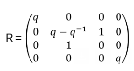
For N=2, i.e. for the basis e₁⊗e₁, e₁⊗e₂, e₂⊗e₁, e₂⊗e₂, R is derived as follows:
Column 1: apply b to e₁⊗e₁ (case a = b = 1): R(e1⊗e1)=q⋅e1⊗e1. In coordinates: (q, 0, 0, 0)ᵀ
Column 2: e₁⊗e₂ (case a=1 < b=2): R(e1⊗e2)=e2⊗e1+(q-q−1)e1⊗e2. In coordinates: (0, q-1, 1, 0)ᵀ
Column 3: e₂⊗e₁ (case a=2 > b=1): R(e2⊗e1)=e1⊗e2, (0, 1, 0, 0)ᵀ
Column 4: e₂⊗e₂ (case a = b = 2): R(e2⊗e2)=q⋅e2⊗e2, (0, 0, 0, q)ᵀ
Hence:
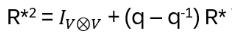
a) The Hecke relation (R – q)(R + q-1) = 0
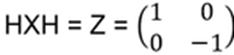
Think of a block diagonal matrix acting on R⁴ = R²⊕R²:M acts on the first R² purely via A, and on the second R² purely via B. The 4×4 Hecke matrix is similar, but with three decoupled blocks acting independently on three invariant subspaces. The 2×2 block in the middle is the only non-trivial one. Hence it sufficient to look at
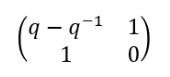
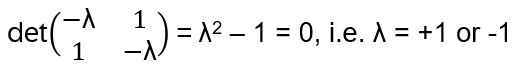
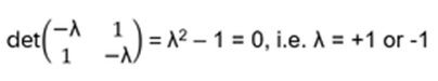
The characteristic polynomial (see Appendix C):
det(λ⋅I−b)=λ(λ−(q−q−1))−1 =λ2−(q−q−1)λ−1
Now factoring for the roots q and -q⁻¹:
(λ−q)(λ+q−1)=λ2+q−1λ−qλ−1=λ2−(q−q−1)λ−1
This shows that the characteristic polynomial is
(λ−q)(λ+q−1)=0
By Cayley-Hamilton (again, Appendix C), R satisfies its own characteristic polynomial on every block:
(R−q)(R+q−1)=0
For the sake of completeness, consider ea⊗ea: R acts as a scalar q, so:
(R – q)(R + q⁻¹)(ea⊗ea) = (q – q)(q + q⁻¹) · ea⊗ea = 0
Therefore the Hecke relation holds. Next:
b) The Braid relation Rᵢ Rᵢ₊₁ Rᵢ = Rᵢ₊₁ Rᵢ Rᵢ₊₁
The Braid relation acts on V⊗V⊗V. Writing Ř₁ = Ř⊗Id and Ř₂ = Id⊗Ř, show
Ř₁ Ř₂ Ř₁ = Ř₂ Ř₁ Ř₂
Check on the basis vectors ea⊗eb⊗c, a < b < c (all distinct)
Left side Ř₁Ř₂Ř₁:
Ř₁ gives ea⊗eb⊗ec → eb⊗ea⊗ec+(q−q-1)ea⊗eb⊗ec
Now Ř₂, with a<c and b<c:
eb⊗ec⊗ea+(q−q-1)eb⊗ea⊗ec+(q−q-1)ea⊗ec⊗eb+(q−q-1)2ea⊗eb⊗ec
Ř₁ again:
ec⊗eb⊗ea +(q−q-1)eb⊗ec⊗ea +(q−q-1)ea⊗eb⊗ec+(q−q-1)ec⊗ea⊗eb+(q−q-1)2ea⊗ec⊗eb+(q−q-1)eb⊗ea⊗ec+(q−q-1)2ea⊗eb⊗ec
Right side Ř₂Ř₁Ř₂:
Forgetting my home page introduction, as one easily shows … 😊: calculating Ř₂Ř₁Ř₂ gives exactly the same ‚q-terms‘!
The mixed cases (with equal indices, or mixed ordering) all work similarly — the (q-q-1) correction terms cancel precisely because of the Hecke relation, ensuring the Yang-Baxter equation holds!
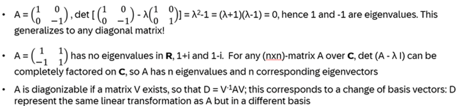
Appendix C: Cayley-Hamilton Theorem
For any square matrix A with characteristic polynomial p(λ), it holds p(A) = 0
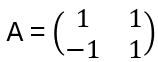
Instead of a proof, lets give an example:
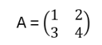
p(λ)=det(λI−A)=(λ−1)(λ−4)−6=λ2−5λ−2
A2−5A−2I= … = 0, as indicated by the theorem
Sources
[1] ‚Topological quantum computation with anyons‚ by Paquette
[2] ‚Aharonov-Bohm interference and the evolution of phase jumps in fractional quantum Hall Fabry-Perot interferometers based on bi-layer graphene‚ by Kim et al., 2024
[3] ‚Braiding Operators are Universal Quantum Gates‚ by Kauffman et al., 2004
[4] ‚What is a Braid Group? ‚ by Glasscock, 2012
[5] ‚Annals of Mathematics: Theory of Braids‚ by Artin, 1947
[6] ‘Quantum Groups in Two-dimensional Physics’ by Gomez et al., Cambridge University Press 1996
[7] ‚Affine Lie Algebras and Quantum Groups‘, by Fuchs, Cambridge University Press 1992
[8] ‚Introduction to Cosets‚ (provided by the American Mathematical Society)