Getting Started – Some Math, 1- & 2-Qubit States and Basic Quantum Circuits

1. Introduction
   • Double Split Experiment
   • RSA, Shors Algorithm and Secrets
2. Mathematical & Quantum Physics Preliminaries
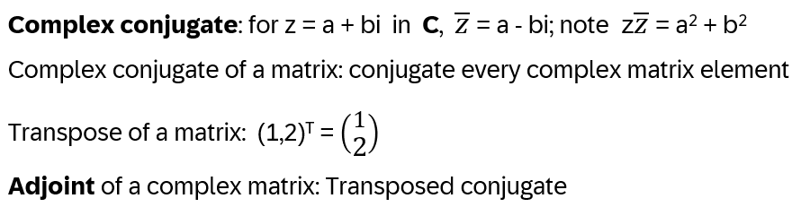
   • a) Some Properties of Complex Numbers
   • b) Linear Transformations and (Unitary) Matrices
   • c) Some Geometry
   • d) Some Group Theory
   • e) Eigenvalues and Eigenvectors
   • f) Tensorproducts
   • g) Root of Unity & Summation Formula
3. One Qubit
   • a) Bloch Sphere
   • b) Bra and Kets
   • c) Quantum State of a Qubit
   • d) Observables and Expectations
   • e) Quantum Gates
4. Two Qubits
   • a) Entanglement
   • c) Multi-Qubit Gates: The Quantum H^{⨂ n} Gate
   • d) The Quantum CNOT/CX Gate
5. Circuits
   • a) Simple Circuits
   • b) Amplitude Maximization & Interference
   • c) Inversion About The Mean
6. Sources

1. Introduction

Note: most of the pictures are generated with Claude.ai

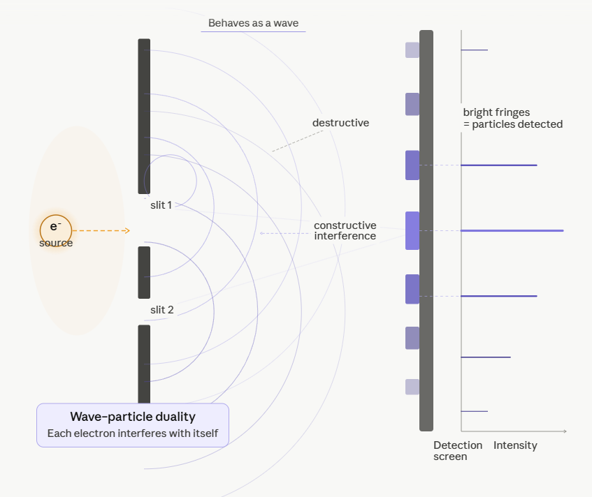
Double Split Experiment – The Importance of Measurement

Wave-particle-duality of light: if not measured through which split the photon is travelling, it behaves like waves, i.e. the interference pattern looks like

But if looked up, it behaves like a particle!

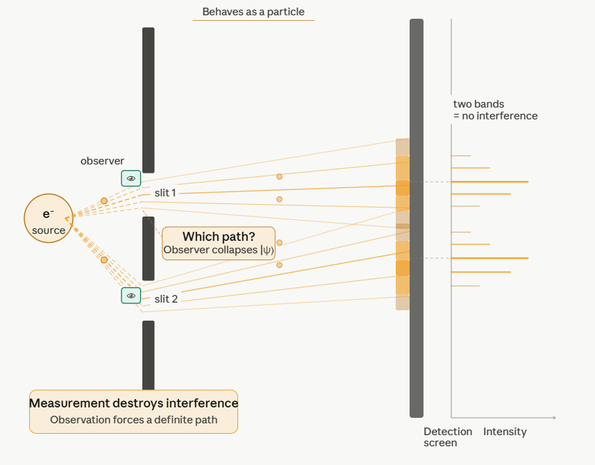
In general: on a very small scale, the world behaves not very intuitive …. (Quantum Mechanics, Quantum Electrodynamics (Photons), Quantum Chromodynamics (Quarks), Supersymmetric String Theory, Quantum Groups, …)

RSA, Shors Algorithm and Secrets

‘Polynomial-Time Algorithms for Prime Factorization and Discrete Logarithms on a Quantum Computer’ by Peter Shor, 1994, [1]

The described quantum algorithm can ‘efficiently’ factor large integers – something classical computer struggle with

Many of todays encryption systems, including RSA (Rivest–Shamir–Adleman), rely on the difficulty of integer factorization.

‘Harvest now, decrypt later’ (HNDL), see e.g. a whitepaper from Mastercard(!) from 2025: ‘Migration to post quantum cryptography – white paper’, [2]

On a more general note: when do quantum algorithms start to outperform classical ones? See e.g. [3]

2. Mathematical & Quantum Physics Preliminaries

This is by no means a thoroughly introduction into the topics, more a mentioning what will be needed

a) Some Properties of Complex Numbers

b) Linear Transformations and (Unitary) Matrices, [4]

• Let U_n and V_m be vector spaces over R of dimension n, m respectively. Let u₁ and u₂ be in U and s₁ and s₂ in R. The function L: U -> V is a linear map if L(u₁ + u₂) = L(u₁) + L(u₂)  and L(s₁u₁) = s₁L(u₁). When U = V, L is called a linear transformation of U

• Assume L(u₁) = Au₁, where A is a n x m matrix:  L(u₁+u₂) = A(u₁+u₂) = Au₁ + Au₂  and L(s₁u₁) = A(s₁u₁) = s₁Au₁, hence the matrix A is a linear transformation

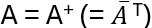
•What are the characteristics of linear transformations that preserve the length, i.e. ||Lv|| = ||v||? They are unitary:

A complex square matrix U is unitary if

with the adjoint matrix

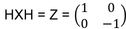
Remark: The matrices corresponding to gates/operations on qubits are all unitary! Examples: Pauli matrices

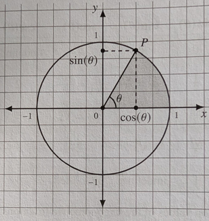
c) Some Geometry

Polar coordinates:     P = r cos(θ) + r sin (θ)

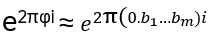
Eulers formula in C:  z = r cos (θ) + r sin(θ) = r e^θi , 0 ≤ θ < 2π

Also: z = r e^2πφi , 0 ≤ φ < 1

Binary form: (used later as approximation of φ)

Base 10:  1/4 + 1/8 = 0.375₁₀

In base 2: 0 x 2^-1 + 1 x 2^-2 + 1 x 2^-3 = .011₂

Another example: 0.2 has no exact finite binary expansion, but repeating decimals: 

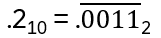
Note: a base 10 rational number has either a finite binary expansion or repeats in blocks, with the repeating block being a base 10 rational number In general: φ ≈ b₁2^-1 + … + b_m2^-m =: (0.b₁b₂..b_m)₂ , hence

d) Some* Group Theory

A collection of objects or transformations with an operation * is called a group if it holds

• Closure

• Associativity

• Unique identity element

• For every object in G exists a unique inverse

If in addition a*b = b*a, G is a commutative or abelian group

Examples: (R,+) is an abelian group, (N,+) is not. Often symmetry operations form a group (e.g. the Bloch sphere representation of quantum states, see later)

*Some more: the (finite) monster ( https://plus.maths.org/content/enormous-theorem-classification-finite-simple-groups ) in the moonshine 😊 ( https://www.quantamagazine.org/mathematicians-chase-moonshine-string-theory-connections-20150312/ )

e) Eigenvalues and Eigenvectors [5]

nxn matrix A: if Av = λv, v is an eigenvector of A and λ the corresponding eigenvalue;  (A – λ I) v = 0 and since v ≠ 0: (A – λ I) not invertible and hence det (A – λ I) = 0

hence 1 and -1 are eigenvalues. This generalizes to any diagonal matrix!

has no eigenvalues in R, 1+i and 1-i.  For any (nxn)-matrix A over C, det (A – λ I) can be completely factored on C, so A has n eigenvalues and n corresponding eigenvectors

A is diagonizable if a matrix V exists, so that D = V^-1AV; this corresponds to a change of basis vectors: D represents the same linear transformation as A but in a different basis

Now a complex matrix is diagonizable if all its eigenvalues are different (in case of repeated eigenvalues it may still be possible, but not in general)

Spectral theorem: A nxn complex matrix A is Hermitian if

Then all eigenvalues of A are real and the corresponding eigenvectors build an orthogonal basis of Cⁿ

Be U a complex unitary matrix:  U = V⁺DV with V and D unitary. Since V⁺=V^-1: VU⁺V = D. In other words: there is a unitary change of basis so that U is diagonal

Note: Solving the eigenvalue problem in quantum mechanics means finding the state (eigenfunction/-vector) the particle can occupy and the physical quantities (eigenvalues) it can possess in that state

f) Tensorproduct

V, W are two finite dimensional vector spaces: V ⨂ W is generated by addition and scalar multiplication of all formal objects v ⨂ w for each v in V and w in W

 If {v1,…vn} and {w1,…,wn} are bases for V and W, then {v₁ ⨂ w₁, …, v_n ⨂ w_m} are basis vectors of V ⨂ W

X, Y are two additional vector spaces, if f: V -> X and g: W -> Y are linear mappings, then so is

      f ⨂ g: V ⨂W -> X ⨂ Y with (f ⨂ g)(v ⨂ w) = f(v) ⨂ g(w)

For 2×2 matrices:

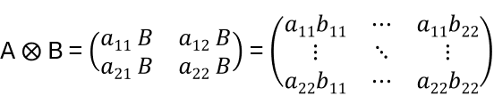
For vectors: v = (v₁,v_2,v₃), w = (w₁, w₂):  v ⨂ w = (v₁w₁,v₁w₂, …,v₃w₂)

For R² ⨂ R² or C² ⨂ C²: e₁ ⨂ e₁ = (1,0) ⨂ (1,0) = (1,0,0,0), … , e₂ ⨂ e₂ = (0,0,0,1). Note: C² ⨂ C² ⨂ C² has dimension 2³

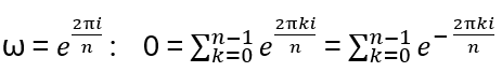
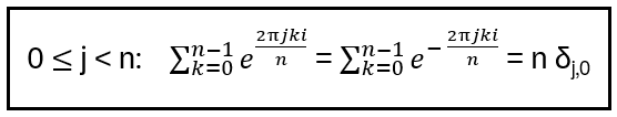
g) Root of Unity & Summation Formula

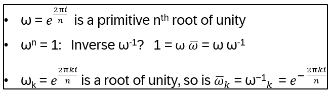
n in N, then the n^th root of unity is ω in C with ωⁿ=1. There are n n^th roots of unity and 1 is always one of them.

ω is a primitive n^th root of unity, if every other root of unity can be written as ω^k for some k in N

Example: all roots of unity for n = 3?

n = 1:  One first root of unity, 1

n = 2:  Two second roots of unity, 1 and -1

n = 3:  With Euler’s formula e^φi = cos(φ) + sin(φ)i, |e^φi| = 1 (note that φ = 2π/3 is a 1/3 rotation around the unit circle), third roots of unity:

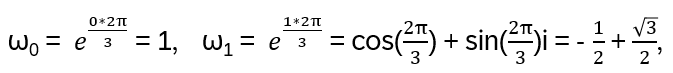
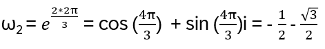
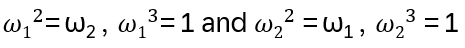
Because 3 is prime, ω is primitive:

In general: 

Now:

xⁿ – 1 = (x-1) (x^n-1 + x^n-2 + … + x + 1)

For every n^th root of unity:  xⁿ – 1 = 0 ,  hence from the above 

x = ω = 1 and for ω ≠ 1: 

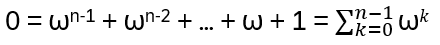
With  

(adding the same set of roots in a different order!)

With the Kronecker delta function  δ_j,k = 0 if j ≠ k and 1 if j = k:

Extended summation formula:

3. One Qubit

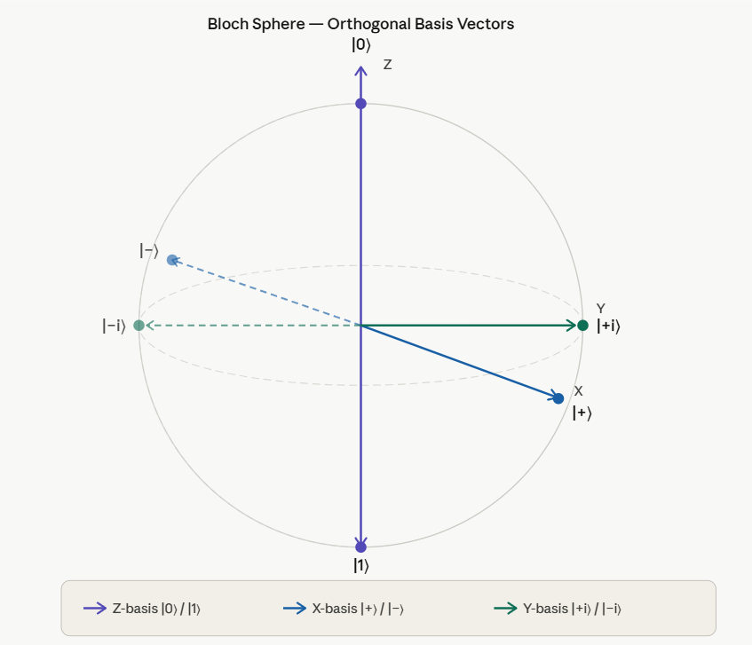
a) Bloch Sphere

A classical bit is 0 or 1 and only in one of those states at any given time!

Qubit representation on the Bloch sphere:

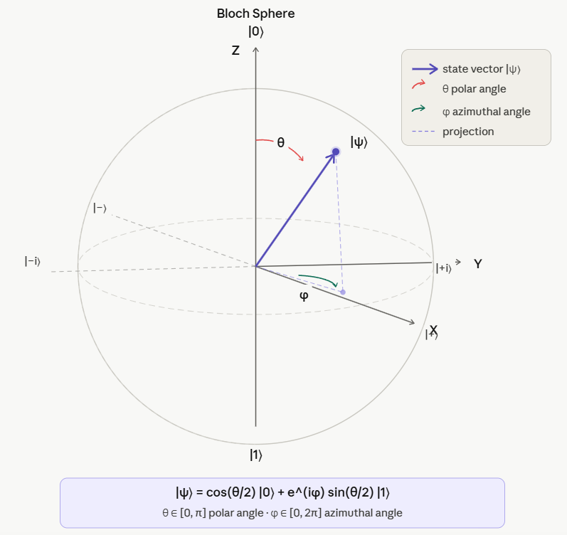
When measured, a qubit is always in states |0> or |1>, but during computing it can be in any (quantum) state on the sphere!

Formally: the qubit is in superposition of |0> and |1> in C² ,

  |ψ> = a |0> + b |1>

with |a|² + |b|² = 1 (unit sphere), where a, b are probability amplitudes

Because qubits are not ‘independent’ to each other as classical bits (superposition of quantum states), huge parallelism is possible.

A single computation acting on 300 qubits can achieve the same effect as 2³⁰⁰ simultaneous computations acting on classical bits!

b) Quantum Mechanics Notification: Bra and Kets

What are |0> and |1>? 

For a vector v, write bra

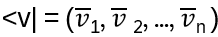
and for w, ket

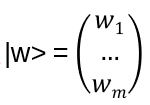
Then for example:   

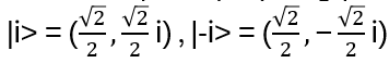
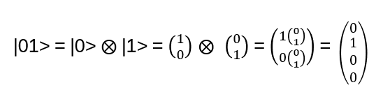
|0> and |1> build the standard orthonormal basis for C²:  |0> = (1,0) = e₁, |1> = (0,1) = e₂ . Other orthonormal basises are 

and

A qubit state has length 1, and any linear transformation must preserve this length! Hence all matrix representations of such transformations are unitary (and hence invertible).

See later for ‘quantum circuits’: all ‘gates’ (operations = linear transformations) are reversible! Only the measurement operation is not! In other words: a quantum circuit is applying unitary matrices to vectors, representing qubit states

c) Quantum State of a Qubit

Quantum state:   |ψ> = a |0> + b |1>  with  ||ψ|| = < ψ | ψ >² = 1

|ψ> = a |0> + b |1> =  r₁ e^φ’i |0> + r₂ e^φ’’i |1>  =  e^φ’i (r₁ |0> + r₂ e^{(φ’-φ’’)i} |1>

Multiplying |ψ> by a phase e^φ’i  doesn’t change it in the sense that the probability of obtaining |0> or |1> is not changed, i.e. there is no observable difference! Hence there are two degrees of freedom for a qubit:

1)Magnitudes r₁, r₂ with r₁²+r₂² = 1

2)Relative phase φ = φ₁ – φ₂

|ψ> of a single qubit is therefore  |ψ> =  r₁ |0> + r₂ e^φi |1> with  r₁, r₂ in R,  r₁²+r₂² = 1,  0 ≤ φ < 2π

d) Observables and Expectations

Measurement of a quantum system:

1. The measurement of a specific observable can be represented by a unitary operator U (matrix)
2. The quantum system is described by a Hilbert-Vector |ψ>
3. A measurement is the application of U to |ψ>
4. Results of the measurement are Eigenvalues u_i of U
5. Probability for a specific u_i: | <u_i| ψ> |²

Let M₀ = |0><0| , M₁ = |1><1| , |ψ> = a |0> + b |1>

  < ψ| M₀ | ψ> = |a|²    probability for |0>

  < ψ| M₁ | ψ> = |b|²    probability for |1>

M₀ and M₁ are observables! The ‘expectation’ <A> of an observable A given the state | ψ> is < ψ| A| ψ>

e) Quantum Gates

Remember: The matrices corresponding to gates/operations on qubits are all unitary!

Examples:

Quantum X Gate                      

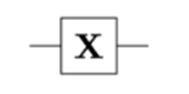
corresponds to the Pauli matrix

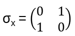
σ_x |0> = |1> ,  σ_x 1> = |0>, i.e. the ‘not’ gate

Bloch sphere: a quantum state is rotated around the x-axis by π. Rotation around the y-axis  σ_y ,  around the z-axis σ_z

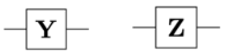
Hadamard Gate

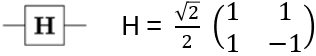
H changes the basis from  |0>,  |1>  to   |+>,  |->

The Quantum R^z_φ Gates: generalize σ_x to 

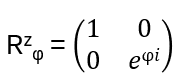
and define

Then: S|0> = |0>,  S|1> =  e^{(π /2)i} |1> = i |1>,  |1> is an eigenvector of S with eigenvalue i

4. Two Qubits

a) Entanglement

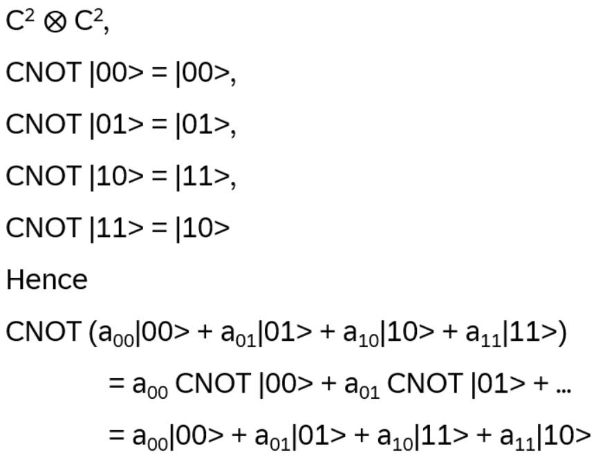
2 qubits q₁, q₂ are in superposition states represented in C² ⨂ C² by a linear combination of |00>, |01>, |10>, |11> (corresponds to 4 possible outcomes of measurement, since each qubit will drop to |0> or |1>)

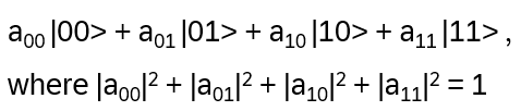
and e.g.

Through measurement the qubits are irreversible projected to |00>, |01>, |10> or |11> with probability |a₀₀|² , |a₀₁|² , |a₁₀|² , |a₁₁|²  respectively. Entanglement is one of the main differences to classical computing! Why? Let’s do an example of Entanglement:

Let q₁, q₂ be in the state

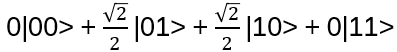
i.e. when measured (very often) it will be half of the time in |01> and half of the time in |10>, but never in |00> or |11>

Now measure q₂ only and let’s say the result is |1>. This can come only from |01> or |11>, but |11> is impossible, hence q₁ must be |0>! This is ENTANGLEMENT

A 2-bit quantum state |ψ> in C² ⨂ C² is entangled if and only if it cannot be written as a tensor of two 1-qubit kets: If

then |ψ> is not entangled

For the example above: assume it is entangled, then there are a₁, b₁, a₂, b₂ in C, with

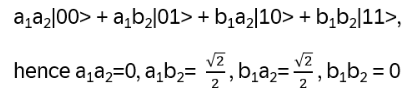
Hence:

-> assumption not correct!

This can be generalized to n-qubit systems with states having 2ⁿ dimensions and the state space can be written as (C²)^{⨂ n}

b) Multi-Qubit Gates: The Quantum H^{⨂ n} Gate

For 2 qubits, quantum gate operations are 4×4 unitary square matrices (for 10 qubits: 2¹⁰x2¹⁰ matrices). 2 Examples:

First the quantum H^{⨂ n} gate

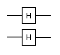
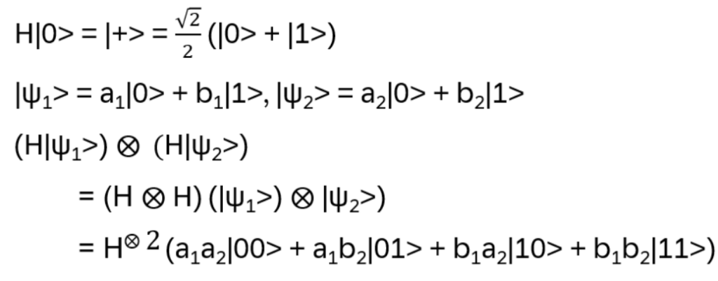
with

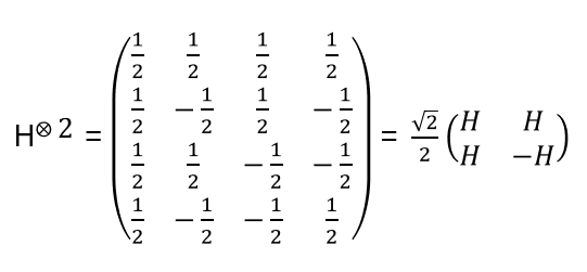
This matrix puts both initialized qubits into a balanced (equal amplitudes) superposition!

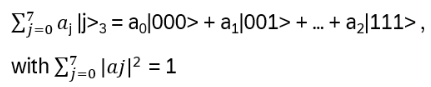
Notation: the set of n-qubits for (C²)^⨂n composed of only 0s and 1s are called computational bases. E.g. for C² ⨂ C² ⨂ C² |000>, |001>, |010>, |011>, |100>, |101>, |110>, |111>. These are the same as |0>₃     |1>₃     |2>₃     |3>₃     |4>₃     |5>₃     |6>₃     |7>₃

For 3-qubits: 

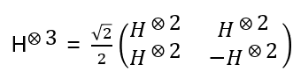
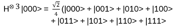
with

beeing a normalization constant

Classical: three bits have 2³ states, but only one at a time. The 3-qubit state H^⨂3|0>₃ contains all 8 possible basis kets at the same time!

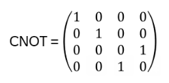
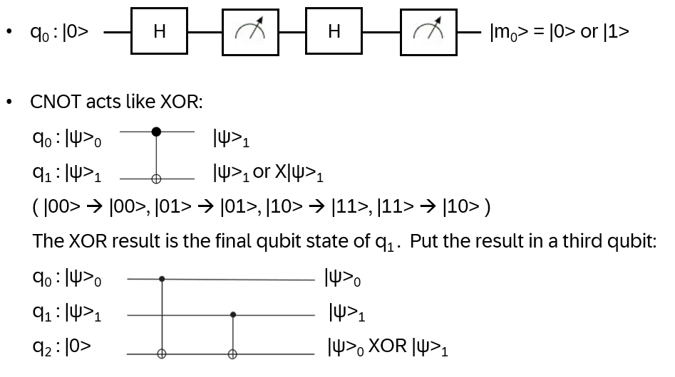
c) The quantum CNOT or CX gate

Now the second gate:

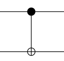
This gate creates entangled qubits (!), ‘C’ stands for ‘CONTROLLED’ (black dot, control qubit; the other: target)

Two input states |ψ₁>, |ψ₂> and hence two outputs (reversable):

• if |ψ₁> = |1> -> output: |ψ₁>,  X|ψ₂>

• if |ψ₁> = |0> -> output: |ψ₁>,  |ψ₂>

Example:

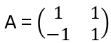
Eigenvalues and Eigenstates of CNOT:

Eigenstates of the Pauli X (bit-flip) operator in the |0>, |1> basis (also called Z basis):

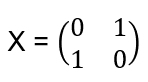
To find the eigenvalues: det(X−λI)=0  

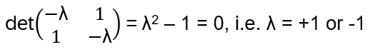
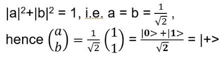
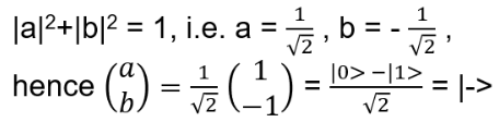
Eigenvectors, ∣ψ> = a|0> + b|1>

i) λ = +1: (X−I) ∣ψ> = 0, hence a = b; normalizing:

ii) λ = -1: (X+I) ∣ψ> = 0, hence a = -b; normalizing:

Behavior X operator:

• X|+⟩ = +|+⟩ (unchanged)

• X|−⟩ = −|−⟩ (phase flip)

• X|0⟩ = |1⟩ (bit flip)

• X|1⟩ = |0⟩ (bit flip)

Note: ∣+> = H∣0> and  ∣−> = H∣1>, and in addition

i.e. H rotates the eigenstates of X onto the eigenstates of Z; |+>, |-> is also referred as X basis

5. Circuits

a) Simple Circuits

Quantum register: a collection of qubits used for computation, all qubits in a register are initialized to |0>

Quantum circuit: a sequence of gates applied to one or more qubits in a quantum register

Simple circuits:

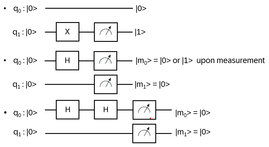
Note: there is no CLONE gate that can duplicate the quantum state of a qubit! (No backups for qubits!)

b) Amplitude Maximization & Interference

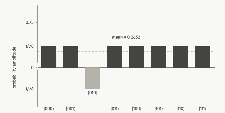
3-qubit quantum register state:

Balanced superposition (all coefficients are equal):   

Let’s assume one of the basis kets is the solution to some problem. Possibility of an amplitude amplification for that ket?  For a quantum algorithm in general: have the results of the final qubit measurements to correspond with high probability to the best solution

How? First: flip the sign of the ket in question (e.g. |010> by U_|010> being I₈ except that the (3,3) entry is -1)

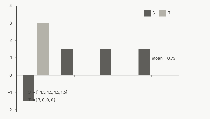
c) Inversion about the mean

Next: inversion about the mean

S = {s_j} finite in R, m the mean of those numbers. Create T = {t_j = 2m – s_j}. Then it holds:

•The mean is still m

•The mapping is reversible

•S_j=m ,  then t_j = s_j = m

•T_j – m = m –s_j

•S_j < m:   t_j > m ,  and s_j > m:   t_j < m

Example: S = {-1,5; 1,5; 1,5; 1,5} -> m = 0,75, T = {3; 0; 0; 0}

Now back to  |φ> = H^{⨂ 3} |000>; define

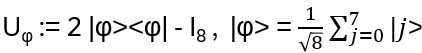
Then U_φ performs an inversion about the mean!

Negating the amplitude and applying U_φ multiple times leads to an increase of the desired probability

But: one can’t apply those two steps too many times, because at some point the desired amplitude is decreasing and the others are increasing again!

Note:

• How many times to maximize the probability? Approximation:  

• Generalization of U_φ:  Groover diffusion operator   H^{⨂ n}( 2 |0>^⨂n <0|^⨂n  –   I^{⨂ n} )H^⨂n

In this context often used:

Oracle function for some question := black box resulting in 1 for yes and 0 for no; oracles cannot answer random questions, they respond to specific queries.

For classical data: f:{0,1}ⁿ -> {0,1}; for quantum computing for basis kets it could be e.g. f(|x>_i) = |1> for one special |x>_i, |0> otherwise. f can be represented by a unitary operator U_f (see the blog about Simon’s Algorithm for an detailed example of how an oracle is working)

6. Sources

[1] ‚Polynomial-Time Algorithms for Prime Factorization and Discrete Logarithms on a Quantum Computer‘ by Shor, 1995 (https://www.arxiv.org/abs/quant-ph/9508027)

[2] ‚Migration-to-post-quantum-cryptography-WhitePaper‚ by Mastercard, 2025

[3] ‚Multi-objective optimization offers bold new path to quantum advantage‘ by Woerner et al. (IBM Quantum Blog), 2026(https://www.ibm.com/quantum/blog/multi-objective-optimization)

[4] Lineare Algebra, Gerd Fischer, vieweg studium, 9. Aufl. 1989

[5] Vorlesungen über Physik, Band III: Quantenmechanik, Feynman/Leighton/Sands, Oldenbourg, 2.Aufl. 1992

‚Dancing with Qubits‘, R.S. Sutor, <packt>, second edition, 2024