Simon’s Algorithm

• Simon’s Algorithm – The Problem
• Circuit
• Analyse the Circuit and the Result
• Appendix A: Complexity of Algorithms
• Appendix B: Complexity Classes
• Appendix C: Hadamard Calculations
• Appendix D: Auxiliary Calculation regarding the component-wise XOR
• Appendix E: The probability of success in Simon’s problem
• Sources

Simon’s Algorithm – The Problem

How can quantum computing bring a real advantage compared to classical approaches? Sometimes the answer could be more difficult as expected: ‚Dequantization‘ describes, under which conditions classical algorithms achieve a performance comparable to quantum algorithms, see e.g. [1] 

Nevertheless: Simon’s algorithm is an early example (1994) of how a quantum algorithm has an exponential improvement over the classial approach. The problem reads as

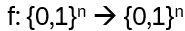
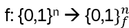
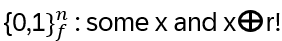
takes a binary string of length n to another such binary string (doesn’t make too much sense, but anyway 😊). When is f(x) = f(y)? In general, this is not known. Therefore, restrict the functions by imposing an additional requirement:

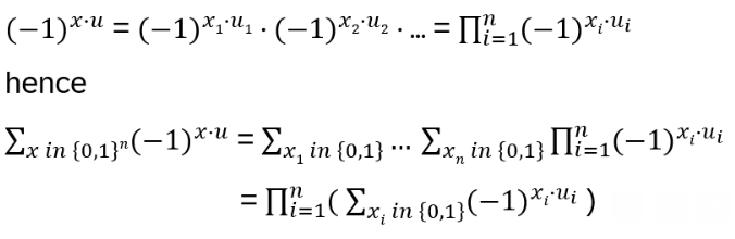
 What does it mean? E.g. for the first component: 

OR

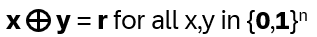
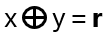
if and only if there is a nonzero string r in {0,1}ⁿ for which

So, what is r?  Classically by brute force:

possible values to consider, so at best (refinement, optimizations) it is

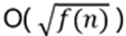
i.e. exponentially hard (see Appendix B). Simon’s algorithm: O(n), i.e. linear in n (see Appendix A)!

Since r has n bits, we need at least n qubits to represent the answer of what is r

Circuit

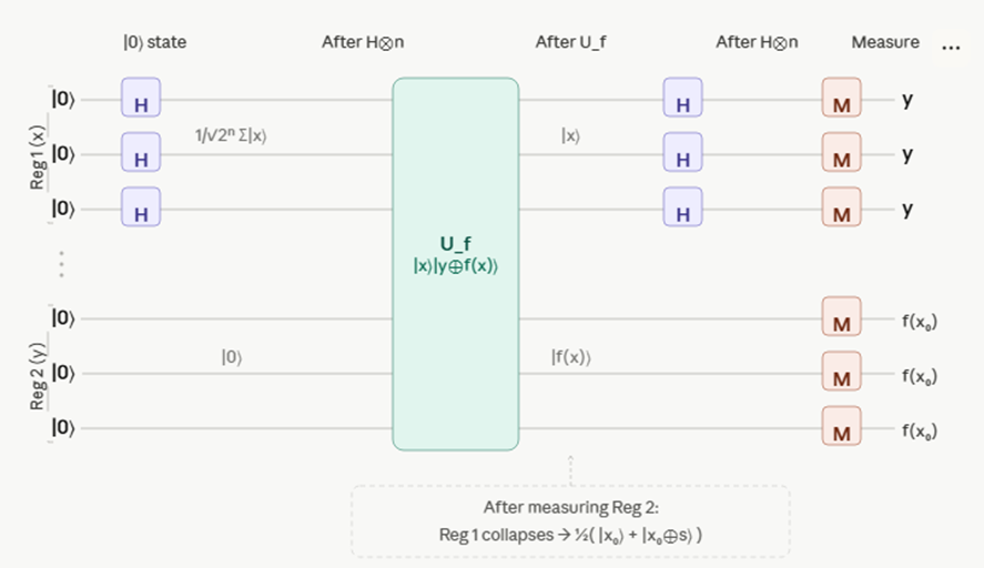
Essentially H-gates and some Oracle function, 2n qubits. As we will see: the register 2’s role is to be entangled with the first register in order to encode information about r (via U_f) into the phase of register 1 and in the end to be measured in order to force the collapse into some quantum state and releasing this information about r with the first register

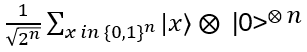
• Initial state: |0>^⨂n ⨂ |0>^⨂n  Applying H gives a balanced superposition of the first n qubits (the last n qubits are still in the initial state):   

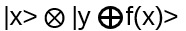
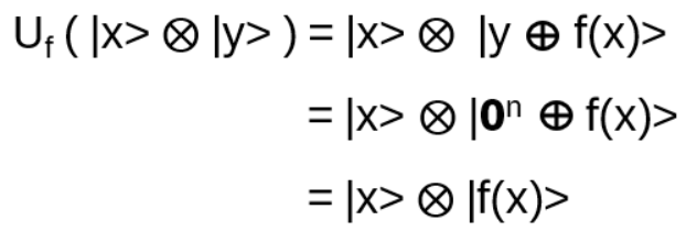
• The input to U_f is |x>⨂ |y>, the output

Apply U_f :

• Apply H to the first n qubits results in

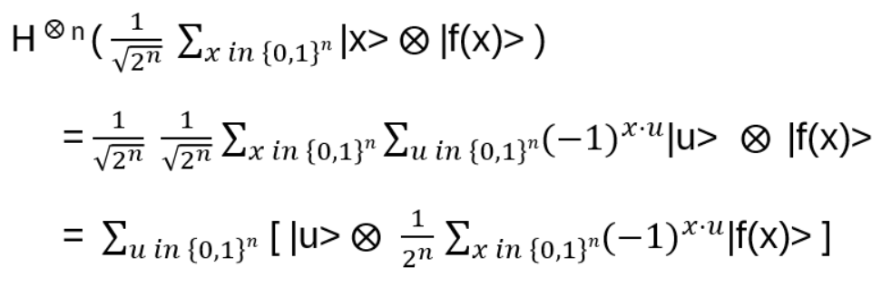
(see Appendix C)

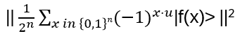
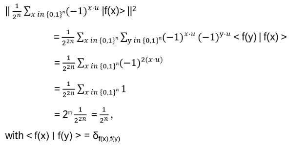
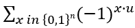
Probability for observing a particular |u>: 

It will be shown, f(x) entangles the U_f-input |x> (uniform superposition of the first n qubits after the first H) with the second register, and by this information about r is created in the phase of the quantum state which can be measured!

Analyse the circuit and the result

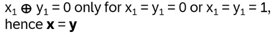
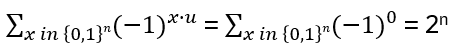
First consider r = 0:

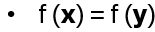
hence x and y are both 0 or 1. Hence the sum over all x equals the sum over all f(x), just in another order! With x = y:

Seeing any of the

values of |u> when measured is

If the circuit is measured many times and sees this distribution of the |u>, r might be 0

Now consider r not equal 0:

Then f is two-to-one:

with x₁ and y₁ are either 0 and 1 or 1 and 0.

Hence: x ≠ y, but f(x) = f(y) for some r: for

exactly two values from {0,1}ⁿ are mapped via f to

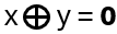
Too see this: the inverse of XOR is XOR itself:

But this looks like f(x) = f(x+r), which implies a periodic function with period r, i.e. f is repeating itself  after r values (e.g. cos(x) = cos(x+r) with r = 2π)

Probability of observing a particular |u> (note that Appendix D is used in the third line):

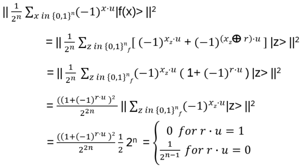
The uniform distribution of kets on all |u> is such that u ∙ r = 0. Suppose we execute the circuit quite often and measure n-1 binary strings u₁, …, u_n-1 . Assume(!) u_k are linearly independent vectors:

u₁ ∙ r = u₂ ∙ r =  … u_n-1 ∙ r = 0

Because of the linear independency it follows, that those n-1 equations are uniquely solvable for (r₁, …, r_n) = r (Gaussian elimination, 0 is the n^th column)

What time does it take to find those n independent u_k among the 2ⁿ binary n-strings?

Finding n linearly independent strings in a collection of n+k nonzero binary n-strings produced by the circuit is

(see Appendix E)

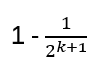
Hence by e.g. choosing k = 30, the chance of failure is less than 1:10⁹! In other words, running the circuit n+30 times gives nearly the probability of 1 to correctly determine r. Hence: O(n)!

QED

(quod erat demonstrandum, not Quantum Electrodynamics 😊)

Appendix A: Complexity of Algorithms

a) If an algorithm is of

with t some number > 1, then the algorithm is of ‘polynomial time’

b) An algorithm of O( f(n) ) can be improved quadratically, if it can be replaced by one of 

c) Exponential improvement: O(log f(n) )

d) Example: an algorithm takes

days to complete (~2740 years). Quadratic improvement: 103 days (~2,74 years), exponential improvement: 6 days!

Appendix B: Complexity Classes

Complexity class P are all problems solvable in

with a deterministic algorithm (vs. a nondeterministic algorithm involving probabilities)

The class NP are all problems whose solution can be checked in

If P = NP is not known!

Example: it is not known if there is a deterministic way of factoring a composite integer (a positive integer greater than 1 that has more than two factors; the smallest one is 4) in

But if known, the check is just multiplying those numbers. Hence deterministic factoring is in NP, but maybe not in P

There are (many) more classes, just two of them: assume P ≠ NP:

NP-Hard: problems at least as hard to solve as the most difficult ones in NP

NP-Complete: a NP-Hard problem can be reduced with an

algorithm to a NP problem

O( f(n) ): number of operations ≤ c f(n).  The problem is at most as hard as c f(n) 

O'( f(n) ): number of operations ≥ c f(n).  The problem is at least as hard as c f(n)

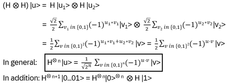
Appendix C: Hadamard Calculation

Recall:

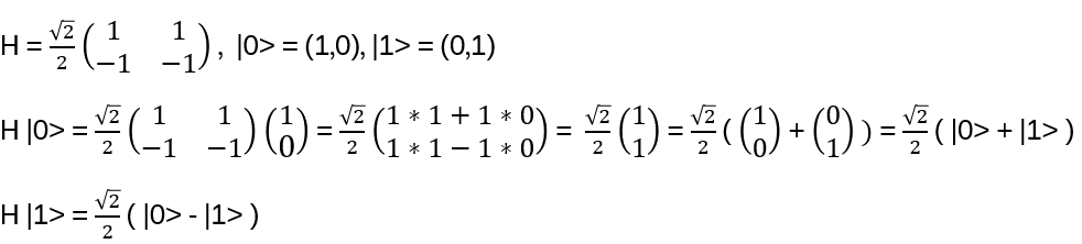
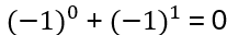
Consider |u>, u = 0 or 1:

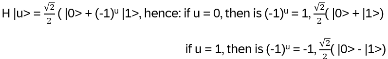
Hence it can be written as: 

Note: the powers of -1 changes the signs of the kets, called phase change.

For bit strings of length 2, i.e. from

the basis kets are |00>, |01>, |10>, |11> := |u> = |u1u2>. With that:

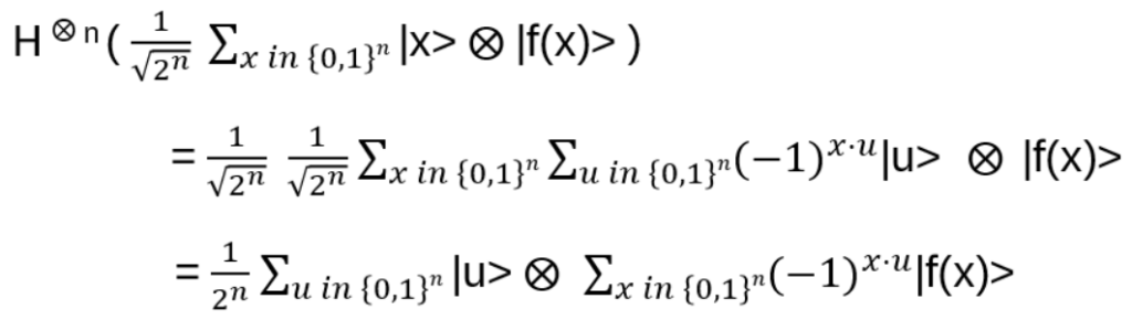
Start the circuit:

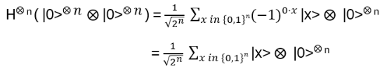
Now apply U_f:  

Finally, H again on the first n qubits:

Appendix D: Auxiliary Calculation regarding the component-wise XOR

If u is the zero-bit string:

All other cases: assume first a single u_k = 1, the rest of the string are 0’s

x in {0,1}ⁿ corresponds to every possible binary string, and each bit x_i goes independently over {0,1}, Hence:

For all i ≠ k: u_i = 0, hence

For i = k:  u_k = 1, hence

hence the product is 0. This can be generalized:

gives 0 for any non-zero u!

Appendix E: The probability of success in Simon’s problem [2]

Each appliance of U_f gives a random vector y satisfying r·u = 0 mod 2. The solution space, i.e. all vectors orthogonal to r, forms a subspace of dimension n−1. To recover r uniquely, one needs n−1 linearly independent equations

A set of n+x random vectors from a (n-1) dimensional subspace of an n-dimensional vector space (with components restricted to 0 and 1) will at some point contain with high probability a linearly independent subset!

Now arrange a matrix with n+x rows (coming from n+x measurements) and n-1 columns (being the desired number of linearly independent vectors)

Now one can formulate two equivalent questions:

• Among the n+x row vectors (each (n−1)-dimensional), do some n−1 of them form a linearly independent set?

• Are all n−1 column vectors (each (n+x)-dimensional) linearly independent?

Due to the rank theorem they have the same answer!

(rank theorem:  

i) the row rank is the maximum number of linearly independent rows

ii) the column rank is the maximum number of linearly independent columns

iii) it holds: for any matrix M: „row rank“=“column rank“ (for proof see e.g. [3])

)

So intuitively, the rows are measured, but the columns are ‘easier’ to analyze:

Pick any column vector. The probability of being non-zero is 

(that a specific bit of the chosen string is 0 has probability 1/2  independently of all other bits). Take this string as a first basis vector.

Now recall that here everything is mod2, that means for the subspace spanned by this first basis vector:

{c · v, c in {0,1}, v being the first column basis vector}, i.e. the subspace contains only two vectors: c = 0 is the zero vector and c = 1 is the vector itself! This holds for all n+x dimensions, hence there are

vectors in total

Therefore, the probability of a randomly selected second column vector to be linearly independent of the first is

Continuing this argument for all n-1 columns give

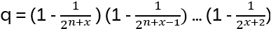
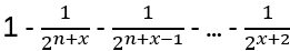
What is a ‘helpful’ lower bound for q (q representing now the probability that there are n-1 linearly independent vectors)? For non-negative numbers a, b, c, … whose sum is less than 1 it holds (1-a) (1-b) (1-c) … exceeds 1 – (a + b +c …), hence

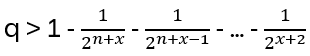
and furthermore (Weierstrass product inequality)

(The last step intuitively:

is greater than 2 times summing the largest minus term …)

So, finally e.g. for x = 20:  q > 0,9999995 that the n-1 vectors are linearly independent.

Intuitively, why only such a small number of additional measurements? Again, this is essentially because of the mod 2: with growing x the (dimension fixed-) subspace containing

vectors gets much smaller than the total subspace of

vectors and with growing x it becomes more and more unlikely that a randomly selected column vector lands in the subspace

Sources

• [1] ‚A quantum-inspired classical algorithm for recommendation systems‘ by Tang, 2019  (arxiv.org/pdf/1807.04271)
• [2] Quantum Computer Science An Introduction by N. David Mermin, Cambridge University Press, 2007,  Appendix G
• [3] ‚Rank–nullity theorem‘, Wikipedia (https://en.wikipedia.org/wiki/Rank-nullity_theorem)
• ‚Dancing with Qubits‘, R.S. Sutor, <packt>, second edition, 2024