- Lie Algebras
- Representations of Lie Algebras
- Modules of Lie Algebras
- Hopf Algebras
- Quantum Groups
- Deformation of Enveloping Algebras
- Example: Uq(sl2)
- Universal R-Matrix – Quantum Double Construction
- Example: Uq(sl2) – continued
- Recovery of the Hecke algebra
- Appendix A: Lie Groups vs. Lie Algebras
- Sources
Lie Algebras [1]
We have to begin with a rush through Lie algebras. Start with some (actually a lot) definitions, concentrating on the terms and defintions we need later: an algebra is a vector space endowed with a bilinear operation · : a x a → a. Equivalently one can define an algebra as a ring (a, ·, +) with the scalar multiplication in R or C (in general: in a Field F)
A Lie algebra is an algebra such that the map [ , ]: g x g → g holds:
•[x,x] = 0 for all x in g (antisymmetry)
•[x,[y,z]] + [y,[z,y]] + [z,[x,y]] = 0 for all x,y,z in g (Jacobi identity)
Antsymmetric, because 0 = [x+y,x+y] = [x,x] + [x,y] + [y,x] + [y,y] → [x,y] = – [y,x]
B be a basis of g: B = {Ta, with a = 1, …, d}, where a = dim g is the dimension of the vector space g. The Ts are the generators of the algebra. Expanding [ , ] into the basis B: [Ta,Tb] = fabc Tc, with fabc in F. The f’s are called structure constants of the Lie algebra
From any associative algebra, i.e. a · (b · c) = (a · b) · c, one can construct a Lie algebra g(a) = (a, [ , ]) by defining [a,b] = a · b – b · a. An example is the Lie Algebra of NxN matrices, with · being the ordinary matrix multiplication
The center Z(g) of a Lie algebra is the set of all elements of g, for which Z(g) = {x in g: [x,g] = 0}
The centralizer of a subset k of a Lie algebra g is the set Cg(k) = {x in g: [x,k] = 0}
A Lie subgroup h of the Lie algebra g is a subvectorspace h ⊆ g which is itself a Lie algebra. An ideal h of the Lie algebra g is a subalgebra with [g,h] ⊆ h. If h and k are ideals, so is [h,k], with [h,k] = spanF{[x,y]: x in h, y in k}
The derived algebra of g is the subspace spanned by all Lie brackets of pairs of elements of g: g’ = [g,g] = spanF{[x,y]: x,y in g}. Note: g’ = [g,g], g’’ = [g’,g’], … If (and only if) this series eventually reaches 0, the corresponding Lie algebra is called solvable. A maximal solvable subalgebra of a Lie algebra g is called Borel subalgebra
An abelian Lie algebra is one, whose derived algebra vanishes, [g,g] = 0. An abelian Lie algebra equals its own center Z(g)
A simple Lie algebra is a Lie algebra which contains no proper ideals (proper: not equal to 0 or g itself) and which is not abelian. Hence in particular for simple Lie algebras: g’ = g
Now the connection to vector spaces:
The direct sum of Lie algebras, g = g1 ⊕ g2 ⊕ … ⊕ gn, is by definition the direct sum of the vector spaces gi with the bracket defined by [x,y] = [x,y]i for x,y in gi (i = 1, ..n) and [gi,gj] = 0 for i ≠ j (i,j = 1, …, n)
In particular: if g = h ⊕ k, h and k are ideals of g!
With that: for a proper ideal k of g define the quotient g/k as the restriction of g to the part not containing k. In other words: if B is a basis of g and B’ ⊂ B a basis of k, then the vector space g/k is generated by the basis B/B’ and the bracket of g/k is obtained from the bracket of g by removing the part not in g/k: [x+k,y+k] = [x,y] + k for all x,y in g/k.
This only works if k is an ideal: for a,b in k [x+a,y+b] = [x,y] + [x,b] + [a,y] + [a,b]. Hence, to be well-defined, [x,b] + [a,y] + [a,b] needs to be in k for all x,y in g. This is true if [g,k] ⊆ k
By construction, g/k is a subalgebra of g. For any ideal k ⊆ g, the Lie algebra g can be written as (g/k) ⊕ k
A semisimple Lie algebra is an algebra which is the direct sum of simple Lie algebras
A reductive Lie algebra is an algebra which is the direct sum of a semisimple and an abelian Lie algebra
What we will see later: Quantum Groups are (Drinfeld–Jimbo) deformations of universal enveloping algebras of semisimple Lie algebras, depending on a parameter q. As q→1, one recovers U(g). And every quantum group is a Hopf algebra
Now consider a specific basis for describing Lie algebras. For semisimple Lie algebras choose the Cartan-Weyl basis, defined as follows:
Choose a maximal set of generators Hi of g so that [Hi,Hj] = 0, for i,j = 1, …, r. Then g0 = spanC{Hi: i = 1, .., r} is a maximal abelian subalgebra of g (Cartan subalgebra). It holds: dim (g0) := rank(g) = r (rank(g) defined as the dimension of the Cartan subalgebra for a given Lie algebra)
A derivation of a Lie algebra δ is a linear map obeying the Leibniz rule: [x,y] → δ([x,y]) = [x,δ(y)] + [δ(x),y] for all x,y in g. An example is the left multiplication: adx:g → g, with y → adx(y) := [x,y] for all y in g (because with this the Leibnitz rule just becomes the Jacobi identity).
For an arbitrary Lie algebra r, the adjoint representation is given by Rad: g → gl(g), with x → adx. Since adx is a derivation, Rad(g) of g under the adjoint representation is a subalgebra Der(g) of all derivations of g
In g0 the adjoint representation splits up into a direct sum of 1-dimensional representations a: g = ⊕ga, with ga = {x in g: adH(x) = a(H) · x for all H in g0}. I.e. for a given g0, the remaining generators can be chosen as eigenvectors of g0 in the sense [Hi, Ea] = ai Ea for i = 1, …, r. The r-dimensional vector (ai) of eigenvalues is called a root of g and ⊕ga the root space decomposition of g relative to g0
Why roots? Since for any H of g0, the complex number a(H) are the non-zero eigenvalues of adH with the characteristic equation det(x – a(H) · I) = 0
Example: sl2(C) (all 2×2complex matrices with trace zero). The algebra sl2 has basis

with brackets [H,E]=2E, [H,F]=−2F, [E,F]=H. The Cartan subalgebra g0 has to be abelian and maximal. Looking at the [ , ] of the basis in sl2, no two basis elements commute, and hence the largest abelian subalgebras are 1-dimensional. Therefore they are spanned by a single generator, choose H: g0 = CH. Now any 1-dimensional vector space is isomorphic to its field, here C, and therefore CH = zH → z in C. To find the roots, one has to check for H in g0: [H,E] and [H,F], which gives the roots 2 and -2 from the [ , ] relations. Hence the root space decomposition becomes
g = g-2⊕g0⊕g2
Let’s proceed by defining the Cartan-Weyl basis as a basis of the semisimple Lie algebra g of the form B = {Hi: i = 1, …, r} ∪ {Ea: a in the set of all roots of g := Θ}
Θs , the set of all simple roots ai (cannot be represented by other roots with positive coefficients) is independent of the chosen basis and exactly of size rank(g), spanCΘs = spanCΘ. Θs is generically not orthonormal. Denoting by ( , ) the scalar product in the root space induced by its Euclidean metric, define:
The Cartan matrix A(g) of the semisimple Lie algebra g is the r x r matrix with elements
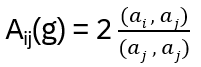
Since the simple roots form a basis, the Cartan matrix is not degenerate (i.e. det(A) is not zero and hence A is invertible). All elements of A(g) are integers, called Cartan integers
Example: sl2(C) again. Θ ={2, -2}, and only a single simple root, Θs = {2}. Therefore the Cartan matrix is 1×1 and A11(sl2) = 2
Note:
•In general one has to introduce coroots, dual spaces and Killing forms, but for the sl2 example it is not needed and hence I omitted it here (I guess there are enough definitions, although the dual space will be introduced later … 😐)
•Any Cartan matrix consists of only 2s as diagonal elements! So the really interesting part are actually the off-diagonal values …
With this define a semisimple Lie algebra in more detail as before:
The semisimple Lie algebra g(Θs) associated to a set Θs = {ai: i = 1, …, r} of r roots ai is uniquely determined by:
There are 3 generators {E±i , Hi: i = 1, …, r} ∪ {1} modulo the relations
•[Hi,Hj] = 0
•[Hi, E±j] = ±Aij E±j , Aij the rxr – Cartan matrix
•[E+i,E–j] = δij Hi
•The generators E±i obey the Jacobi identity
•(adE±i )1-Aij E±j = 0
The last relation fixes the length of the ai string through aj. It is called the Serre relation and the full set of relations are the Chevalley-Serre relations. Written out it equals [E±i ,[E±i ,⋯[E±i ,E±j]⋯]] = 0 with 1 – Aij brackets.The Serre relation fixes the length of the ai string through aj.What does this mean exactly?
Fix two roots ai,aj with i≠j. The ai-string through aj is the set of all roots of the form: αj+kαi, k∈Z that actually occur in Φ and is of the form aj−pai, aj−(p−1)ai, …, aj,…, aj+qai for some non-negative integers p and q. It can be shown: p−q=(aj,ai)=Aji! The Serre relation says now, that aj+(1−Aij)ai is not in Φ, i.e. that root does not exist and the string ends with aj+(−Aij)ai = aj+qai. Since aj is simple and positive, p has to be zero and the ai string through aj is aj,aj+ai,…,aj+(−Aij)ai of length 1−Aij. The Serre relation brings together the roots of g with their generators
Note: the only parameters occurring in this definition are the Cartan integers and are together with the relations above sufficient to describe g!
Representations of Lie Algebras
The general linear algebra of a vector space V is the algebra of endomorphisms of V: gl(V) = {ϕ: V → V: ϕ is linear} with [ , ] = gl(V) x gl(V) → gl(V), (ϕ,θ) → [ϕ,θ] = ϕ · θ – θ · ϕ, where · here denotes the composition of maps. gl(V) is a vector space over the field F (same as for V), otherwise the ‘–’ wouldn’t make sense.
Note: gl(V) and End(V) is the same
With this definition, gl(V) is a Lie algebra. gl(V) is isomorphic to glN(V), the set of N x N matrices over F
A representation R of the Lie algebra g is a homomorphism of g into gl(V):
R: g → gl(V) with [x,y] → R([x,y]) = R(x) · R(y) – R(y) · R(x) for all x,y in g
While in g there is no definition of a product other than the Lie bracket, for R one has the matrix multiplication, hence one can define arbitrary power series in the elements of R. Replacing formally R(x) by x, one can define the universal enveloping algebra U(g) of a Lie algebra, which consists of all finite (formal) power series of the elements of g. Note that U(g) is associative, and hence not a Lie algebra itself
Example: Consider the 3-dimensional Lie algebra U, V, W with [U,V] = W, [U,W] = [V,W] = 0. The derived algebra is 1 dimensional and hence abelian and solvable. A matrix representation is

Modules of Lie Algebras
A module of the Lie algebra g is a vector space V (over the same F as g) together with an action of g on V with
• : g x V → V with the properties (a,b in F, x,y in g, v,w in V):
(ax + by) • w = a (x • w) + b (y • w)
x • (av + bw) = a ( x • v) + b (x • w)
[x,y] • w = x • (y • w) – y • (x • w)
The dimension of a g-module is the dimension of the underlying vector space.
What is the connection between representations and modules?
Given a representation R: g → gl(V), V becomes a module g via defining x • w = (R(x)) (w); remember that R(x) is an endomorphism on w in V (if R is represented by a matrix, one writes R(x) w)
And conversely: for a g-module V, a representation R of g is defined by (R(x)) (w) = x • w
A submodule is a subset which is a module in itself. With this two additional definitions:
An irreducible module of a Lie algebra is a module with no proper submodules
A fully reducible module of a Lie algebra is a module which is the direct sum of irreducible modules
How do the last two definitions translate to representations?
A presentation R of g is irreducible if and only if the image R(g) is simple.
Note: from a reducible module which is not fully reducible, one can derive a fully reducible module by a quotient in analogy to algebras
If g is abelian, the representation matrices R(x) for a fully reducible representation are diagonal matrices!
Hopf Algebra [2]
In order to understand quantum groups, we start even more generic: a Hopf algebra a is a vector space endowed with 5 operations:
•M: a x a → a (multiplication)
•η: F → a (unit map, F the underlying field of the vector space, here C or R)
•∆: a → a x a (co-multiplication)
•ε: a → F (co-unit map)
•γ: a → a (antipode, the ‘inverse’ map)
with the following properties:
•M · (I · M) = M · (M · I) (associativity)
•M · (I · η) = I = M · (η · I) (existence of a unit element)
•(I · ∆) · ∆ = (∆ ·I) · ∆ (co-associativity)
•(ε · I) · ∆ = I = (I · ε) · ∆ (existence of a co-unit)
•M · (I · γ) · ∆ = η · ε = M · (γ · I) · ∆
•∆ · M = (M · M) · (∆ · ∆) (connecting axiom)
Notes:
•Examples: group algebras and universal enveloping algebras U(g) are Hopf algebras
•The concept of co-multiplication arises, because unlike for Lie algebras in general tensor products cannot be defined for associative algebras without additional structure. To see this as an example: let A be an associative algebra and V, W two A-modules. To make V ⊗ W an A-module, try a⋅(v⊗w) := (a⋅v)⊗(a⋅w). But because of a→a⊗a: (λa)⋅(v⊗w) = (λa⋅v)⊗(λa⋅w) = λ2(a⋅v⊗a⋅w) which is not linear!
•The antipode is essentially a way of connecting multiplication and co-multiplication in a non-trivial way
•When a basis {ei} is fixed, the Hopf relations can be expressed by structure constants
•With the permutation map π: a x a → a, x⊗y = y⊗x define ∆’ = π · ∆. Then ∆’ is also a (co-associative) co-multiplication (with only the antipode to be modified: γ’ = [γ(a)]-1)
A Hopf algebra is called commutative if and only if M · π = M, π being the permutation map. The Hopf algebra is called co-commutative, if and only if π · ∆ = ∆ (or in other words ∆’ = ∆). An example for a co-commutative algebra is again the enveloping algebra U(g). For any commutative or co-commutative algebra: γ · γ = I
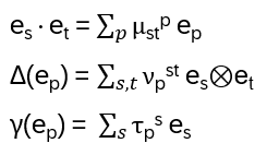
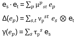
With a fixed basis {ep} and matrices μ , ν ,τ for multiplication, co-multiplication and antipode:
Quantum Groups
Mabe first the disappointing part 😊: after all this …, there is no generally accepted definition of what a quantum group is. But nevertheless: here we will use the following definition as a quasitriangular Hopf algebra. The additional property is shared by quantum universal enveloping algebras and hence those algebras are referred to as quantum groups
And just to mention the light at the end of the tunnel 😊: below we will encounter with those algebras the Yang-Baxter equation, the Braid group, the Hecke algebra and a way of solving the YBE by universal R-matrices! So, let’s see …
A quasitriangular Hopf algebra is a Hopf algebra a for which the co-multiplications ∆ and ∆’ = π · ∆ are related by conjugation: for some element R of a x a, which is invertible, it holds
∆’(x) = R · ∆(x) · R-1 for all x in a (the conjugation) and satisfies in addition
(I · ∆)(R) = R13 · R12 (if R takes the product form R12 = r1 ⊗ r2, R13 = r1 ⊗ e ⊗ r2 and so on …)
(∆ · I)(R) = R13 · R23
(γ · I)(R) = R-1
R-1 of R in a x a is that element of a x a which satisfies R-1 · R = e ⊗ e = R · R-1 (e the unit element). A is called triangular, if and only if R12 · R21 = e ⊗ e or in other words if π(R) = π(r1 ⊗ r2) = R-1
∆’(x) = R · ∆(x) · R-1 in a x a . Embedding this relation in the first components of a x a x a by tensoring with y to the right: ∆’(x) ⊗ y = R · ∆(x) · R-1 ⊗ y. Multiplication in the first two components is independent of the third: ∆’(x) ⊗ y = R12 · ∆(x) · R12-1 ⊗ y. Multiply both sides by R12: (∆’(x) ⊗ y) · R12 = R12 · (∆(x) ⊗ y) and hence with Δ(x)⊗y = Δ(x)⊗I(y) = (Δ · Id)(x⊗y):
R12 · (∆ · I)(x ⊗ y) = (∆’ · I)(x ⊗ y) · R12 for all x ⊗ y in a x a
Taking x ⊗ y = R and with (∆ · I)(R) = R13 · R23 (left side) and in addition for the right side ∆’ = π · ∆ it follows
R12 · R13 · R23 = R23 · R13 · R12
This is the Yang-Baxter equation and R is called universal R-matrix!
And hence we have also a relation of the quasitriangular Hopf algebra with the Braid group via the representation by the YBE
(Trivial) Example: the universal enveloping algebra of any Lie algebra with R = 1⊗1 is a triangular Hopf algebra. Note: this R with Uq(sl2) is not quasitriangular, because of ∆′ ≠ ∆ (not co-commutative)
Deformation of Enveloping Algebras
Recall: the universal enveloping algebra U(g) of a Lie algebra is the algebra of finite (formal) power series in the generators of g
What we will do know: define a quantum group with exactly the generators and relations from the definition of a semisimple Lie algebra (the Chevalley-Serre relations) and deform them by a parameter q. As q → 1, the ‘classical’ relations for a semisimple Lie algebra are recovered from the quantum group
Introduce the following notations for the q-number:
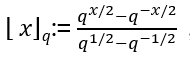

(using L’Hôpital to proof), called deformation of x; note: in the definition of the quasitriangular Hopf algebra we use
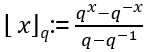
which is just another convention achieved by q→q1/2, but both conventions deliver
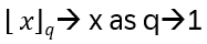
With

define
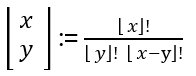
The quantum universal enveloping algebra Uq(g) is the algebra of power series in the 3r+1 generators {E±i, Hi: i = 1, …, r} ∪ {1} modulo the relations
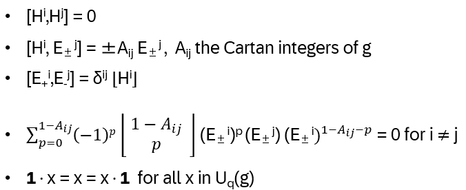
line 4 beeing the q-deformed Serre relation and [x,y] = x · y – y · x for M(x ⊗ y) = x · y (the formal product in U(g))
Notes:
a) [E+i,E–j] = δij ⌊Hi⌋: the classical version of the semisimple Lie algebra was [E+i,E–j] = δij Hi, describing that positive and negative generators from different simple roots commute, and from the same simple root give the Cartan generator Hi
For the quantum version, with K = qH (see also the following example Uq(sl2))

and for i ≠ j this describes again, that simple roots commute: [E+i,E–j] = 0 (because ai – aj is not a root if i ≠ j). For i = j this gives the q-Cartan element ⌊Hi⌋qi : ⌊Hi⌋qi → Hi as qi→1
b) The q-deformed Serre relation: the classical Serre relation is

Note that

with

being the binomial coefficient. Hence the classical expression becomes

How to derive the quantum version? First the q-binomial coefficient: the definition was
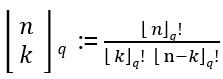
and fulfilling the identity (Pascal’s identity for q-binomials)

leads to the classical expression for q→1
Second the q-adjoint: with the scalar q<ai,aj> defined by Ki E±j Ki−1 = qiaij E±j , aij being the corresponding Cartan matrix entries

I.e. computing
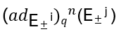
means building all possible strings (E±i)n-k (E±j) (E±i)k and determine the coefficients each one gets. In the quantum case, each time E±j is braided past a power of E±i it picks up a factor qiaij, leading to

Note the relation of Uq(g) with the Braid group:
π (the permutation operator) is an isomorphism of vector spaces V⊗W → W⊗V. This holds e.g. for U(sl2), but not Uq(sl2). There are two paths from V1 ⊗V2 ⊗V3 → V3 ⊗V2 ⊗V1 (i.e. two isomorphisms) and for any two representations V, W of Uq(sl2), the map RV,W : V⊗W ≅ W⊗V holds only, if the two isomorphisms coincide (what we need). This leads to (RV1,V2 ⊗ IV3) · (IV2 ⊗ RV1,V3 ) · (RV2,V3 ⊗ IV1) = (IV1 ⊗ RV2,V3 ) · (RV1,V3 ⊗ IV2) · (IV3 ⊗ RV1,V2), With V1=V2=V3=V this condition reads R1R2R1 = R2R1R2 on V⊗V⊗V, R on V⊗V being the R-matrix associated with the representation of Uq(g). So, for any quantum group and any representation of it, we have a local representation of the Braid group! (see blog ‘Topological Quantum Computing I – Braid Group, Yang-Baxter Equation & Hecke Algebra’)
Example: Uq(sl2) [3], [4], [5]
The Lie algebra sl2 = {A are 2×2 matrices in R: trace(A) = 0} has the following basis in the 3-dimensional vector space (3-dim because: 4 numbers in A minus the trace constraint):

and it holds: [H,E] = 2E, [H,F] = -2F, [E,F] = H. H has integer eigenvalues n. In order to derive Uq(sl2), replace H ‘formally’ with K = qH and its inverse K-1, introducing q. Why in this form? First of all, K are just generators with KK-1 = 1, without the need to explicitly writing down qH. In addition: qH · v = qn · v, whenever H · v = n · v (the integer eigenvalues). And for q→1 : [H,E] = 2E is recovered: [H,E] = 2E yields qH E q−H = q2 E = KEK-1 recovering [H,E] = 2E again for q→1
Note: there are two conventions: K = qH → KEK-1 = q2E (Drinfeld-Jimbo) and K = qH/2 → KEK-1 = qE (‘half-weight’ convention). This is a ‘global’ renormalization, i.e. every relation in K looks a bit different dependent on this choice
The algebra Uq(sl2) is then generated by {H,E, F,} with the relations (using the Drinfeld-Jimbo normalization)
• [H,E] = 2E , [H,F] = -2F , and

• Comultiplication: ∆(H) = H⊗1 +1⊗H, Δ(E) = E⊗qH + 1⊗E, ∆(F) = F⊗1 + q-H⊗F
• Counit: ε(E) = ε(H) = ε(F) = 0, ε(K) = 1
•Antipode: γ(H) = -H, γ(E) = -EK-1, γ(F) = -KF
giving a Hopf algebra structure! Verifications:
a) The coproduct on E is consistent with the relation KEK-1 = q2E: it holds ∆(KEK-1) = q∆(E). LEFT with (A⊗B) (C⊗D) = AC⊗BD:
∆(K) ∆(E) ∆ (K-1) = (K⊗K) (E⊗K + 1⊗E) (K-1⊗K-1) = (KEK-1 ⊗ KKK-1) + (KK-1 ⊗ KEK-1) = q2E⊗K + 1⊗q2E = q2(E ⊗K + 1⊗E) = q2 ∆(E)
b) From the Hopf relations, the antipode has to satisfy [M · (I · γ) · ∆ ](E) = η · ε(E) = 0; with ∆(E) = E⊗K + 1⊗E:
M ⊗ (I ⊗ γ) (E⊗K + 1⊗E) = E · γ(K) + 1 · γ(E) = E K-1 – EK-1 = 0
Note about the quasitriangular q-deformed Serre relation: since Uq(sl2) is of rank 1 (only a single root, with a 1×1 Cartan matrix A11 = 2, hence a i ≠ j relation does not arise (in contrast to e.g. Uq(sl3)).
Universal R-Matrix – Quantum Double Construction
For a an arbitrary Hopf algebra fix a basis {ep} and express the relations by structure constants for the matrices μ for multiplication, ν for comultiplication and τ for the antipode:
Now define the dual space a* (i.e. the space of linear maps φ on a, which inherits a Hopf algebra structure as follows) with a dual basis {ei} defined by ei(ej) = δij. Then all structure relations of H gets dual and swapped:
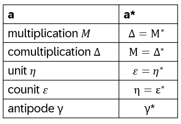
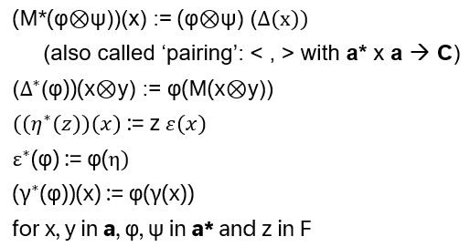
Using the opposite co-multiplication on a*, one gets a new Hopf algebra ao and with matrices μ , ν ,τ for multiplication, co-multiplication and antipode from the Hopf algebra a definition by duality:
- Multiplication:

Then
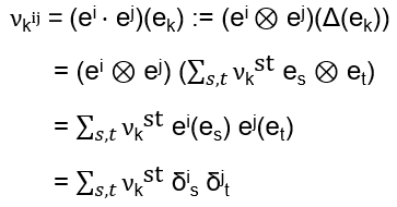
- (Opposite) Comultiplication:

Then

- Unit
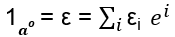
- Counit

Antipode

To any Hopf algebra a one can associate a quasitriangular Hopf algebra d(a), called the double of a, which contains a and ao as Hopf subalgebras. For {es} a basis for a, {es} for ao, define a pairing from the subalgebra structures to describe how elements from a and ao commute past each other as follows:
A dual pairing of a and ao is a bilinear mapping < , >: ao x a → C, such that for all f, f1, f2 in ao and a, a1, a2 in a:
<f,a1a2> = < Δ*(f),a1⊗a2>
<f1f2,a> = <f1⊗f2,Δ(a)>
<f,1a> = ε*(f) , <1a*,a> = ε(a) , < γ(f),a> = <f, γ*(a)>
Now for d(a) = a⊗ao, let {eres} (with eres := (er⊗1)·(1⊗es) = er⊗es) be the basis, then e.g. Δ:d(a)→ d(a)⊗d(a), i.e. the comultiplication becomes a linear combination of tensor products. For d(a) to become an algebra, we need to define the multiplication of elements of a and ao
Co-multiplication:
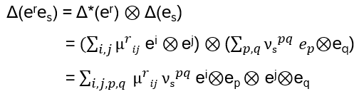
Multiplication:
(eres ⊗ epeq) (ekel ⊗ emen) = (eresekel ⊗ epeqemen)
The universal R-matrix of the quantum double construction lives on d(a) ⊗ d(a):

is in (ao⊗a)⊗(ao⊗a)= d(a)⊗ d(a), also fulfilling (see the definition of quasitriangularity)
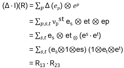
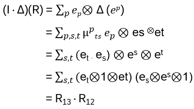
Note: In order to completely describe the multiplication on d(a), what is the relation between the basis {eres} and the basis {eres}? In order to fulfill ∆’(x) = R · ∆(x) · R-1 it holds, [6]: if the multiplication on d(a) is defined to satisfy

d(a) becomes a quasitriangular Hopf algebra with R-matrix as above and

To summarize:
To every Hopf algebra a there is associated a quasi-triangular Hopf algebra that contains a and ao as Hopf subalgebras and is isomorphic to a⊗ao as a vector space
Example Uq(sl2) continued – Universal R-Matrix & Quantum Double Construction
Apply the general results to Uq(sl2). The Chevalley generators E, F, H build a basis {HnEmFl},n,m,l from 0 to ∞ of Uq(sl2) and generate the subalgebras Uq(b+) = span{HnEm} and Uq(b–) = span{HnFm}
Recall: a Borel subalgebra is a maximal solvable subalgebra. For sl2(C), b+ is generated by
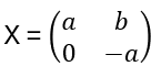
a and b complex numbers (the upper-triangular matrices) and b– by
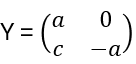
(the lower-triangular matrices)
Note: h being the span of the strictly diagonal matrices, it holds the triangular decomposition: sl2 = b– ⊕ h ⊕ b+
To derive the universal R matrices, we need also the deformed enveloping algebras of the Borel subalgebras:
Uq(b+) = span{Hn Em : n, m ≥0} and Uq(b–) = span{Hm Fl : l, m ≥0} , i.e the algebra of all polynomials in the generators H and E or F respectively
For later reference, for Uq(b–) it holds: [H,F] = -2F, Δ(Ĥ) = Ĥ⊗1+1⊗Ĥ, Δ(F) = F⊗1 + K-1⊗F
The basis of the dual space (Uq(b+))* dual to {Hn Em} is defined by {Ĥn Êm} with the linear functions Ĥ and Ê in (Uq(b+))* defined by acting on the basis H and E as
Ĥ(H) = < Ĥ,H> = 2/lnq, Ê(H) = < Ê,H> = 0, Ĥ(E) = <Ĥ,E> = 0, Ê(E) = < Ê,E> = 1
With K = qH again, choose {Km En} as basis for b+ (the so called PBW basis (Poincare, Birkhoff, Witt)), and hence define Ĥ and Ê by defining the pairing for the dual as < Ĥ, Km En > := 2m δn,0 and < Ê, Km En > := δn,1
Note: the 2/lnq and the 2m δn,0 in the relations are not by accident nor independent, but a specific normalization. In Uq(sl2) we have [H,E] = 2E, with 2 the only simple root of sl2(C). In this sense H gives the Cartan integer A11(sl2) = 2. To mirror that Cartan-like behavior with Ĥ (matching [H,F] = -2F for [Ĥ, Ê]):
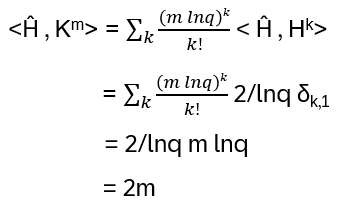
Let’s show the relation < Ĥ, Km En > := 2m δn,0 (the second goes similar) explicitly, using structure constants. By definition with the dual basis being ei: <ei,ej> = δi,j , define for the pairs using the actual basis e(m,n) := Km En leading to <e(m’,n’) , e(m,n)> = δm’m δn’n. Ĥ is not a dual basis element, but a linear combination of them:
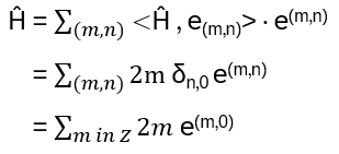
with 2mδn,0 =: cmĤ being the structure constants of Ĥ:
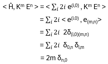
The commutation relations and comultiplication for (Uq(b+))* follow from the duality definition:
[Ĥ, Ê](x) = (M*(Ĥ⊗Ê) – M*(Ê⊗Ĥ)) (x) = (Ĥ⊗Ê – Ê⊗Ĥ)(Δ(x)). Let’s do the terms of individually:
a) Δ(Km En): since Δ is a homomorphism it holds Δ(Km En) = Δ(Km)⋅Δ(En) = Δ(Km) ⋅ Δ(E)n = (Km⊗Km) ⋅ Δ(E)n From above for < Ĥ, Km En > , only n = 0 and n = 1 will contribute and therefore for n = 1:
Δ(Km En ) = (Km⊗Km) ⋅ Δ(E) = (Km⊗Km) (E“⊗“qH + „1⊗“E) = KmE ⊗ Km+1 + Km ⊗ Km E
b) Only n = 1: (Ĥ⊗Ê)(Δ(x) = < Ĥ⊗Ê, Δ(Km En)> = < Ĥ⊗Ê , KmE ⊗ Km+1 + Km ⊗ KmE> = < Ĥ, KmE> < Ê, Km+1> + < Ĥ, Km> < Ê, KmE> and with the ‘δ’ results from before < Ĥ , Km> < Ê, KmE> = 2m ⋅ 1
c) Again, only n = 1 contributes: <Ê⊗Ĥ, Δ(Km En)> = <Ê⊗Ĥ, KmE⊗Km+1 + Km⊗KmE> = < Ê, KmE > < Ĥ, Km+1> + < Ê, Km> < Ĥ, KmE> = < Ê, KmE > < Ĥ, Km+1> = 1 ⋅ 2(m+1)
Bringing it together with: [Ĥ, Ê](Km En) = <[Ĥ, Ê], Km En > = <ĤÊ+ – Ê+Ĥ, Km En > = (2m – 2(m+1))
δn,1 = – 2m δn,1 = -2m <Ê, Km En> and hence [Ĥ, Ê] = – 2Ê
For the dual coproduct
i. Ĥ: (Δ∗(Ĥ))(x⊗y) := φ(M(x⊗y)), i.e. < Δ∗(Ĥ), KnE m⊗KpEr > := < Ĥ, KnEm⊗KpEr >
Ĥ is a linear map and E mKp = q-2mp KpEm (from KEK-1 = q2E), and with < Ĥ, Km En > := 2m δn,0 , m, n ≥ 0 resulting in m=r=0: <Ĥ, Kn⊗Kp > = 2(n + p) = 2n·1 + 1·2p = <Ĥ, Kn >< 1Ĥ, Kp > + < 1Ĥ, Kn >< Ĥ, Kp >, with the counit <1Ĥ,Kn> = ε(Kn) = 1 follows
Δ∗(Ĥ) = Ĥ⊗1+1⊗Ĥ
ii. Again, with KE = q2EK: <Δ∗(Ê), KnEm ⊗ KpEr > := <Ê, Kn(EmKp)Er> = q-2mp <Ê, Kn+p Em+r>. To be non-zero, because of < Ê, Km En > := δn,1 it follows m+r = 1, hence for m=1, r=0 it follows … = q-2p < Ê, Kn+pE>. With
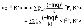
and with <Ĥk, Kn> = (2n)k (by induction from < Ĥ, Km En > := 2m δn,0 ):
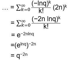
hence q-2p <Ê, Kn+pE> = <Ê, Kn+pE> <q−Ĥ,Kp> → Ê⊗q–Ĥ
In addition, for m=0, r=1: 1· <Ê, Kn+pE> = <1, Kn><Ê,KpE> → 1⊗Ê Adding both terms up gives the result: Δ∗(Ê) = Ê⊗q-Ĥ + 1⊗Ê
Now, define φ: Uq(b–)→ Uq(b+)* with φ(F) = Ê and φ(H) = 2/lnq Ĥ
•[φ(H),φ(F)] = 2/lnq [Ĥ,Ê] = 2/lnq (-lnq Ê) = -2 Ê
•(φ⊗φ) Δb-(H) = (φ⊗φ) (H⊗1+1⊗H) = φ(H)⊗1 + 1+φ(H) = 2/lnq (Ĥ⊗1 + 1⊗Ĥ ) = Δ(Ĥ)
•With φ(K) = elnq φ(H) = e2Ĥ := K’ it follows (φ⊗φ) Δb-(F) = φ(F)⊗1 + φ(K)-1⊗φ(F) = Ê⊗1 + K’⊗Ê. Now with the transposition operator: π(Ê⊗1 + K’⊗Ê) = 1⊗Ê + Ê⊗K’ = Δ(Ê)
So actually φ is a mapping of (φ⊗φ)Δb- to π Δ φ and also holds for (φ⊗φ) Δb-(H):
π(Δ(φ(H))) = lnq/2 1⊗Ĥ + lnq/2 Ĥ⊗1=lnq/2 (Ĥ⊗1+1⊗Ĥ)
Hence φ is an isomorphism with the co-opposite comultiplication of Uq(b+): Uq(b–) ≌ (Uq(b+)*)°and therefore the quantum double d(Uq(b+)) = Uq(b+) ⊗ Uq(b+)°is isomorphic as a vector space to Uq(b+) ⊗ Uq(b–)
Next: with the relation Ĥ = H (i.e., the dual generator equals the original one) generates a two-sided Hopf ideal and the quotient of d(Uq(b+)) by this ideal recovers Uq(sl2)!
d(Uq(b+) = Uq(b+) ⊗ Uq(b–) is generated by {H, E, Ĥ, Ê} with the pairing from before. Then Ĥ – H is an ideal and co-ideal to d(Uq(b+):
a) co-ideal: For a Hopf ideal generated by z it must hold Id = <z> = d(a) z d(a) = xzy for all x,y in d(a). Since d(Uq(b+)) carries the tensor product structure of d(Uq(b+))* and d(Uq(b+))* it holds Δd(Ĥ – H) = (Ĥ – H)⊗1 + 1⊗(Ĥ – H), which is in d(Uq(b+)) . In addition ε(Ĥ – H) = ε(Ĥ) – ε(H) = 0 – 0 = 0, which is together the definition of being Ĥ-H being primitive. This proofs already the co-ideality, because with z = Ĥ-H, x,y in d(Uq(b+)):
Δ(xzy)=Δ(x)(z⊗1+1⊗z)Δ(y)=Δ(x)(z⊗1)Δ(y)+Δ(x)(1⊗z)Δ(y) and writing

leads for the left term of the ‘+’ to

i.e. the element is in (Ĥ – H)⊗ d(Uq(b+)). Analogously the right term, showing Δ(xzy) gives an element of (Ĥ – H)⊗d(Uq(b+)) + d(Uq(b+))⊗(Ĥ – H). In addition: ε(xzy) = ε(x)ε(z)ε(y) = ε(x)⋅0⋅ε(y) = 0
b) ideal: Since Ĥ-H is primitive, it has to be shown [x, Ĥ-H] is in <Ĥ-H> for all generators. [H, Ĥ] = 0, hence [H, Ĥ-H] = 0 and [Ĥ,Ĥ-H] = 0
In addition: [Ĥ, E] = 2E , [H, Ê] = -2Ê
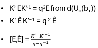
[ To see this: let L = qĤ. Then it holds [E, Ê] = (K-L-1)/(q-q-1) (from [E,F] = (K-K-1)/(q-q-1)) and from Uq(b+) KEK-1 = q2E. With that:
K [E, Ê] K-1 = [KEK−1,KÊK−1]=[q2E, KÊK−1] and

and hence KÊK−1 must be q-2 Ê being equivalent to [H, Ê] = -2Ê . Analogously: LEL-1 = q -2E ]
With that: [E,Ĥ-H] = (-2E) – (-2E) = 0 and [Ê,Ĥ-H] = 0. So Ĥ-H commutes with every generator of d(Uq(b+) (and hence lies in the center of d(Uq(b+))
Therefore, the quotient d(Uq(b+)) / <Ĥ – H> is a well defined Hopf algebra
Now we show, that this quotient is isomorph to Uq(sl2):
Define a quotient map σ: d(Uq(b+)) → d(Uq(b+)) / <Ĥ – H> being a linear map, mapping every element in the double to its equivalence class x’ := x + <Ĥ – H>. We have already seen: every element w from the ideal <Ĥ – H> is mapped to 0: σ(w) = σ(<Ĥ – H>) = 0 and hence σ(Ĥ) – σ(<H>) = 0. Now for any x in d(Uq(b+)) it holds (Ĥ+x’) – (H+x’) = 0 which leads to Ĥ+x’ = H+x’ and so in the quotient group only a single generator H’ = H = Ĥ is needed (also mapping K to L defining K’ in the quotient!). With that in the quotient group it holds
But this are exactly the defining relations of Uq(sl2), i.e d(Uq(b+)) / <Ĥ-H> ≌ Uq(sl2). Now finally we can calculate the R-matrix:
The R-matrix of d(Uq(b+)) is generally given from above as
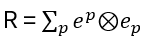
Recall: we want the YBE equation to generate the Hecke algebra connecting the YBE solution to the braid group representation. For any Hopf algebra a, the double d(a) is quasitriangular and the general (formal) form of the universal R-matrix is built from elements of a⊗a* under pairing as d(a)⊗d(a)⊗d(a). For Uq(sl2) we want to derive a specific representation connecting the YBE solutions to anyon braiding. And for this we need the quotient: to see this, recall the triangular matrix decomposition sl2 = b– ⊕ h ⊕ b+ , h being the strictly diagonal matrices. But h exists in b+ and in b– . Hence taking the tensor product, the diagonal matrices are counted twice. This redundancy leads to infinite-dimensional degree of freedom for the R-matrix. By factoring out the overlapping (unrelated!) Cartan eigenvalues from H and Ĥ , the underlying vector space becomes ‘well-defined’ for computing the pairing and derive the universal R-matrix for d(Uq(b+))
Let’s start with the classical double, [7]:
(L, [ , ], φ) be a Lie algebra with [ , ]* : L* x L* à L* defined by [f, g]* = (f⊗g) · φ (where f, g in L*) turns the dual L* of L into a Lie algebra. Consider now the vector space D = L ⊕ L* on which we define the scalar product
<(X, f),(Y, g)> = f(Y) + g(X) for f, g in L* and X, Y in L
Then a unique Lie algebra structure exists on D such that L and L* are Lie subalgebras of D with <[A, B], C> = <A, [B, C]> for all A, B, C in D
With a particular basis {Xj} in L and with the dual basis {fi} (i.e. fi(Xj) = δij) for L* it holds
[Xi,Xj ] = Ckij Xk , [fi,fj] = Γijk fk , [fi,Xj] = Cijk fk − Γikj Xk
The space D together with this Lie algebra structure and the scalar product is called the Double Lie algebra associated to the Lie bi-algebra (L, [., .], φ)
Then: r = Xi⊗fi in D⊗D, called the canonical element, is a solution of the classical Yang-Baxter equation
[r12, r13] + [r12, r23] + [r13, r23] = 0
Proof:
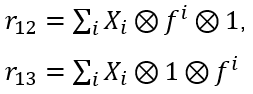

all in U(D)⊗3 with (a⊗b⊗c)(a′ ⊗b′⊗c′ ) = aa′ ⊗b b′ ⊗c c′ . Now:

and similar the other two gives B = CijkXk⊗fi⊗fj + CjkiXi⊗fk⊗fj − ΓjikXi⊗Xk⊗fj + ΓkijXi⊗Xj⊗fk = 0 (recall that for any tensor Γjik summation indices can be arbitrarily renamed) QED
Note:
• Since the co-product of the quantum group Uq(sl2) is not co-commutative (in contrast to U(sl2)), the obtained local representations of the braid group are not trivial (as we will see)
• A universal R-matrix satisfies the ‘flip operator’ ∆’(x) = R · ∆(x) · R-1, the co-algebra homomorphisms (I · ∆)(R) = R13 · R12 and (∆ · I)(R) = R13 · R23 and the YBE R12 · R13 · R23 = R23 · R13 · R12
• Uq(b+) does not possess a universal R-matrix, but building the quasitriangular quantum double does, by deriving it from the non-commutative and non-co-commutative pairing relations
Now let’s calculate the universal R-matrix for the quantum (deformed by q) case, [8]
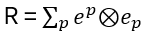
and with a basis change to
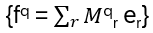
for Uq(b–) this leads to

and Mpq = fp(eq), since er(es) = δrs and with {HkEl} as basis for Uq(b+) and {ĤmÊ n} for Uq(b–), we get from the pairing: Mklmn = <Ĥm Ên,Hk El> = < Ĥm⊗Ên, ∆(Hk El)> = < Ĥm⊗Ên, ∆(Hk) ∆(El)>; note that ∆ maps to a*⊗a, hence for the left part (‘H-part’) with
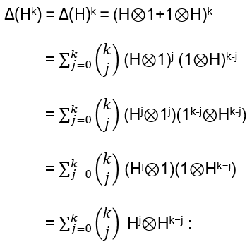
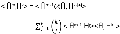
and with k-j=1:

and with <Ĥ0,Hk> = δk,0 and iterating m times gives <Ĥm,Hk> = δk,m m!
For the right part (‘E-part’): K=qH, KEK-1 = q2E, ∆(El) = Δ(E)l = (1⊗E + E⊗qH)l
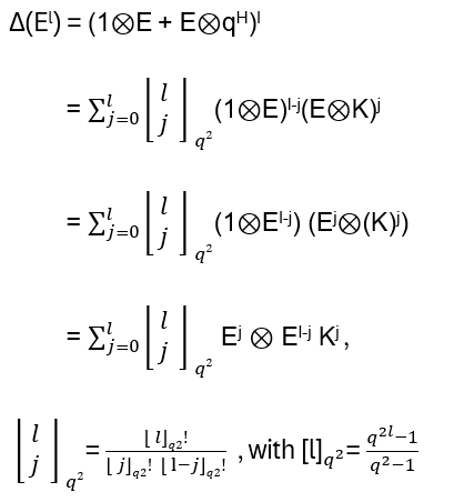
the Gaussian or asymmetric q-integer
Note:

with the definition as before (the ’symmetric form‘):
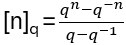
Hence:

and pairing gives

Because of duality of Ĥ and H, as Ê and E: < Ĥm , Hj Ei > = 0 unless i = 0 and therefore <Ên, Hk−j el > = 0 unless k-j = 0, hence
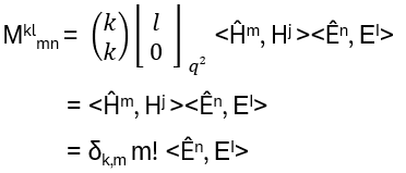
With <Ê, El> = c δl,1 and the pairing <f1f2,a> = <f1⊗f2,Δ(a)>:
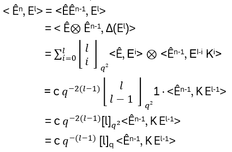
Expand

but <Ên-1, Hael-1> = δa,0 which is 0 for a ≥ 1 , hence

and from the basis definition of the dual pairing <Ên, El> = 0 except for l = n :
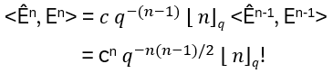
using <Ê0, E0> = 1
Bringing everything together
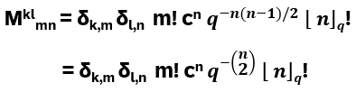
Note: regarding <Ê, El> = c δl,1 , c will be

Without this normalization (i.e. <Ê, El> = δl,1), the off diagonal element of the universal R-matrix for Uq(sl2) would be derived as q-1/2 and with that the derived R-matrix does not fulfill the YBE! The normalization with c= 1/(q-q-1) leads to a valid universal R-matrix, as we will see
Since Mklmn is diagonal, its invertible:
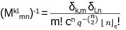
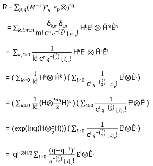
With the 2-dimensional representation of Uq(sl2)
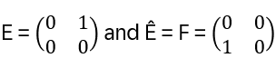
and E2 = F2 = 0 (so only l = 0,1):
R = qH⊗H/2 (1 + (q-q-1) E⊗F)
With {e1, e2} as basis for the underlying vector space V: He1 = e1, He2 = -e2, Ee1 = 0, Ee2 = e1, Fe1 = e2, Fe2 = 0, giving two eigenvalues: h1 = 1, h2 = -1
H⊗H act on V⊗V: (H⊗H) (ei⊗ej) = Hei⊗Hej = hiei⊗hjej = (hihj)ei⊗ej
In the ‘ordered’ basis, (e1⊗e1 , e1⊗e2 , …) are the diagonal elements, hence the Cartan factors on the diagonal are: qH⊗H/2: e1⊗e1 = q1/2 e1⊗e1 , e1⊗e2 = q-1/2 e1⊗e2 , e2⊗e1 = q-1/2 e2⊗e1 , e1⊗e1 = q1/2 e2⊗e2
E⊗F gives a nonzero element only for e2⊗e1: (q-q-1) (E⊗F)(e2⊗e1) = (q-q-1) (e1⊗e2)
Hence e.g. for the third column: qH⊗H/2(1 + (q-q-1) E⊗F)(e2⊗e1) = qH⊗H/2 (e2⊗e1 + (q-q-1) e1⊗e2) = q-1/2(e2⊗e1) + q-1/2 (q-q-1) e1⊗e2)
Putting it together:
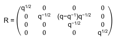
rescaling by q1/2 gives
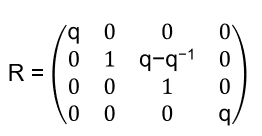
Recovery of the Hecke algebra
From the quasitriangular structure of Uq(sl2), the R-matrix acts on V⊗V in the basis {v+⊗v+, v+⊗v−, v−⊗v+, v−⊗v−}. Define
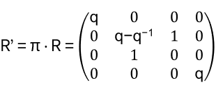
acting on V⊗V → V⊗V. The matrix splits into 1⊕2⊕1 – blocks and hence the eigenvalues are
i) q for v+⊗v+
ii) q for v−⊗v−
iii) q and q-1 for
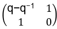
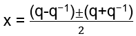
(characteristic polynomial x2-(q-q-1)x -1 = 0, discriminate (q-q-1)2 + 4 = (q+q-1)2, and hence
giving the eigenvalues q and -q-1)
So the characteristic polynomial for R’ is (R’- q)(R’+ q-1) = 0 giving R’2 = (q – q-1)R’ + 1
Define bi = R’i,i+1 acting on the i-th and (i+1)-th vector space of V⊗n, we get bi2 = 1 + (q – q-1)bi
This is the defining relation of Hn(q)! (see the blog ‘Topological Quantum Computing I – Braid Group, Yang-Baxter Equation & Hecke Algebra’)
Also the braid relation and the commutativity holds:
For R it holds R12R13R23 = R23R13R12 and applying π’s one gets R’12R’23R’12 = R’23R’12R’23 which is equivalent in b to bibi+1bi = bi+1bibi+1, which is the braid relation of Hn(q)
For |i – j| ≥ 2 (i.e. ‘distant’ generators), since they act on completely separate tensor factors, it holds bibj = bjbi
These three relations are exactly the defining relations of Hecke algebra, hence giving the connection to the braid group.
Moreover the Hecke algebra is derived purely from the Hopf algebra structure of Uq(sl2)!
Appendix A: Lie Groups vs. Lie Algebras [1]
•The Lie group G is a continuous space of mappings/operators, e.g. all rotations and linear movements in this space. These elements can be smoothly ‘combined’ (multiplication and inversion)
•A Lie algebra is a vector space g with [ , ] satisfying antisymmetry and the Jacobi identity. G is the tangent space at the identity and its elements are infinitesimal (Lie-) generators (moving away from the identity)
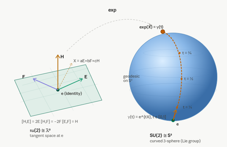
It holds: g in S3, A a matrix in the Lie algebra in R3 for example,
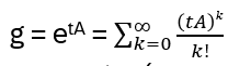
t being a continuous parameter (e.g. a rotation angel)
Hence a scaling factor q on an element X in the Lie group creates on the Lie generators
group: q = ehX → algebra: ln q = h · X
(an vice versa). At the identity h=0, it holds q = I (of the group) and hence
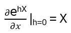
So differentiating the Lie group element at the identity gives X
Sources
[1] ‚Lie Gruppen und Lie Algebren‘ by Hilgert et al., vieweg 1991
[2] ‚Affine Lie Algebras and Quantum Groups‘, by Fuchs, Cambridge University Press 1992
[3] ‚Quantum Groups‚ by Kassel, Springer Verlag 1995
[4] ‚Quantum groups and knot algebra‚ by Dieck, 2004
[5] ‚Hopf Algebras and Representation Theory of Hopf Algebras‚ by Meusburger, 2022
[6] ‚Quasitrangular Hopf algebras and the quantum double‚ by Ram
[7] ‚An introduction to quantized Lie groups and algebras‚ by Tjin, 1991
[8] ‚Fusion for the Yang-Baxter equation and the braid group‚ by Poulain d’Andecy
Schreibe einen Kommentar